Probieren hilft beim Studieren!
Interaktive Vorlesungsfolien im Webbrowser
Lehrstuhl für Computergraphik, TU Dortmund
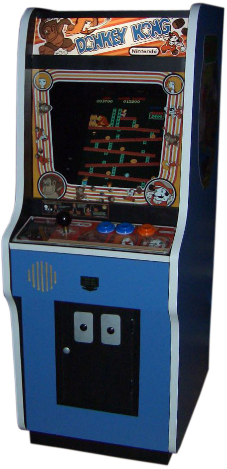
Bilder und Videos
Aufzählungen
- Mario
- Der Held
- Peach
- Die Prinzessin
- Donkey Kong
- Der Böse
 Mario
Mario 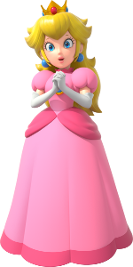 Peach
Peach 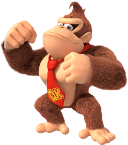 Donkey Kong
Textauszeichnungen
- Mario
- ist fett (gedruckt)
- Prinzessin Peach
- ist hochgestellt
- Donkey Kong
- ist schräg
Mario Peach Donkey Kong
Nummerierungen
- Donkey Kong
- entführt Peach
- Mario
- rettet Peach
- Peach
- findet Mario toll
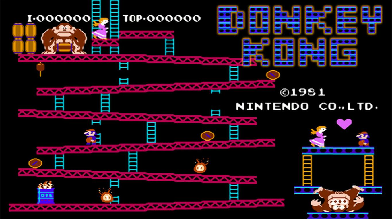
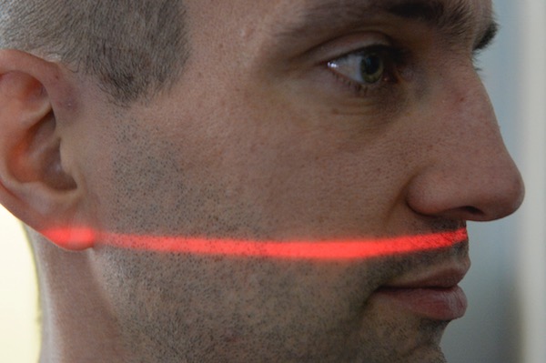
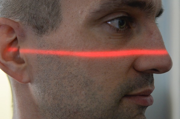
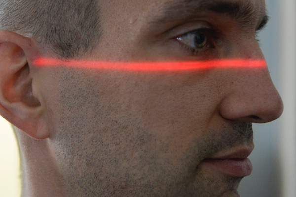
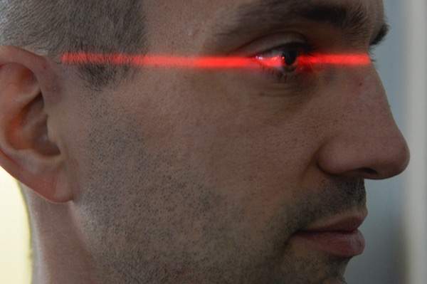
Bild-Sequenzen
Graph-Diagramme mit GraphViz

Diagramme mit Tikz/Latex

Plots mit gnuplot

Audience Response System
Wer bekommt am Ende die Prinzessin?
-
- Nein, der ist böse!
-
- Nein, der lebt unter Wasser!
-
- Nein, den mag keiner!
-
- Klar!
Zuordnungsaufgaben
-
- Prinzessin
-
- Donkey Kong
-
- Supermario
Freitextaufgaben
Wie heißt die Prinzessin?
Selektionsaufgaben
Die Prinzessin ist verliebt in