Discrete Laplacians for General Polygonal and Polyhedral Meshes

Astrid Bunge
TU Dortmund

Marc Alexa
TU Berlin

Mario Botsch
TU Dortmund
Problem Setting
Solve PDEs on surface meshes and volume meshes
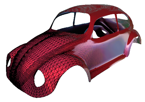 Surface mesh
 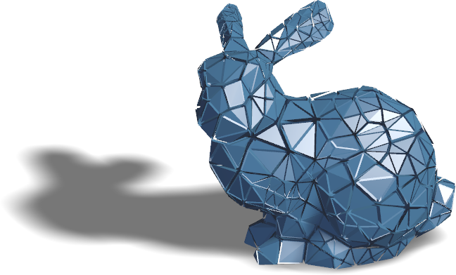 Volume mesh
Discrete Laplacian has various applications
- Mean Curvature
- Smoothing & Fairing
- Parameterization
- Deformation
- Geodesics Distances
- …
Discrete Laplacians for Polygonal/Polyhedral Meshes
Surface Meshes: Triangles Polygons Volume Meshes: Tetrahedra Polyhedra
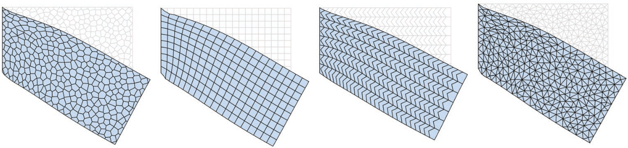
Discrete Laplacians for Polygonal Meshes
Surface Meshes: Triangles Polygons Volume Meshes: Tetrahedra Polyhedra
Triangulate the Polygons?


Triangle Meshes

- Connectivity / Topology
- Vertices \(\mathcal{V} = \{ v_1, \dots, v_n \}\)
- Edges \(\mathcal{E} = \{ e_1, \dots, e_k \}\), \(e_i \in \mathcal{V} \times \mathcal{V}\)
- Faces \(\mathcal{F} = \{ f_1, \dots, f_m \}\), \(f_i \in \mathcal{V} \times \mathcal{V} \times \mathcal{V}\)

- Geometry
- Vertex positions \(\{ \vec{x}_1, \dots, \vec{x}_n \}\), \(\vec{x}_i \in \R^3\)
Functions on Triangle Meshes
- Define a piecewise linear function on a triangle mesh as \[f(\vec{x}) = \sum_{i \in \set{V}} f_i \varphi_i(\vec{x})\]
- Assign function values \(f_i\) to vertices \(v_i\) with positions \(\vec{x}_i\)
- Assign linear “hat” basis functions \(\varphi_i(\vec{x})\) to vertices \(v_i\)
- Equivalent to barycentric interpolation of \(f_i\) within triangles

Laplace Matrix & Mass Matrix
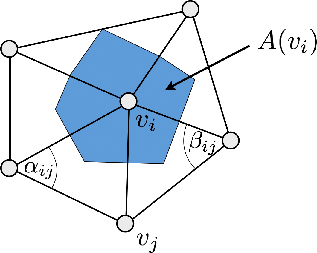
\[ \small \begin{eqnarray*} \mat{L}_{ij} &=& -\int \grad \varphi_i \cdot \grad \varphi_j &=& \begin{cases} \frac{\cot\alpha_{ij}+\cot\beta_{ij}}{2} & \text{if } j\in\set{N}\of{i} \,, \\[0.5em] \displaystyle -\sum_{k\in\set{N}\of{i}} \mat{L}_{ik} & \text{if } j=i \,, \\[0.3em] 0 & \text{otherwise}. \end{cases} \\[1em] \mat{M}_{ij} &=& \int \varphi_i \, \varphi_j &=& \begin{cases} \frac{\abs{t_{ijk}} + \abs{t_{jih}}}{12} & \text{if } j\in\set{N}\of{i}\,, \\[0.5em] \displaystyle \sum_{k\in\set{N}\of{i}} \mat{M}_{ik} & \text{if }j=i \,,\\[0.3em] 0 & \text{otherwise}. \end{cases} \end{eqnarray*} \]
Local to Global Assembly


Properties
- Symmetry
- Locality
- Linear precision
- Negative semi-definiteness
- Null property
- Positive weights

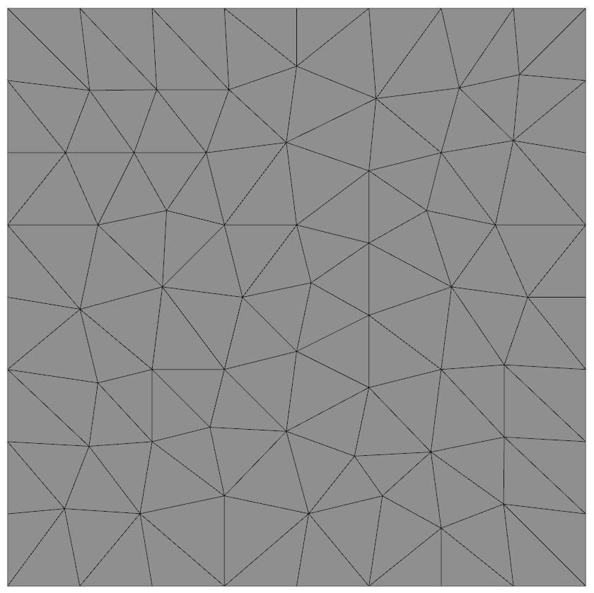
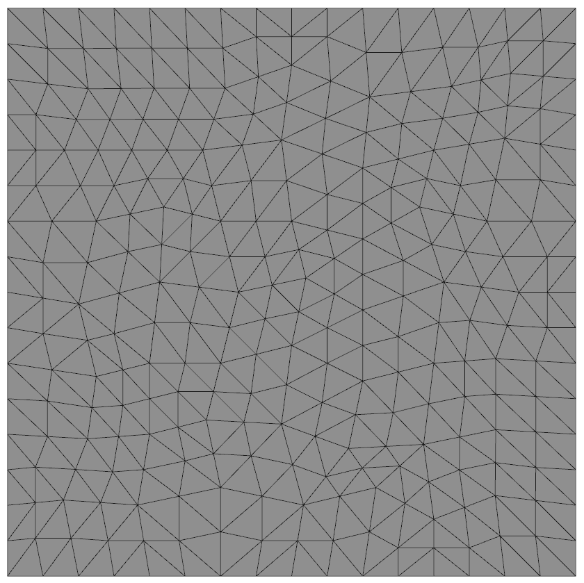
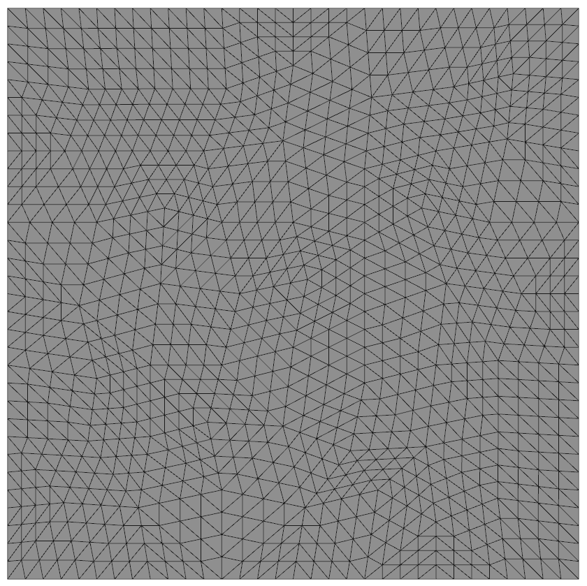
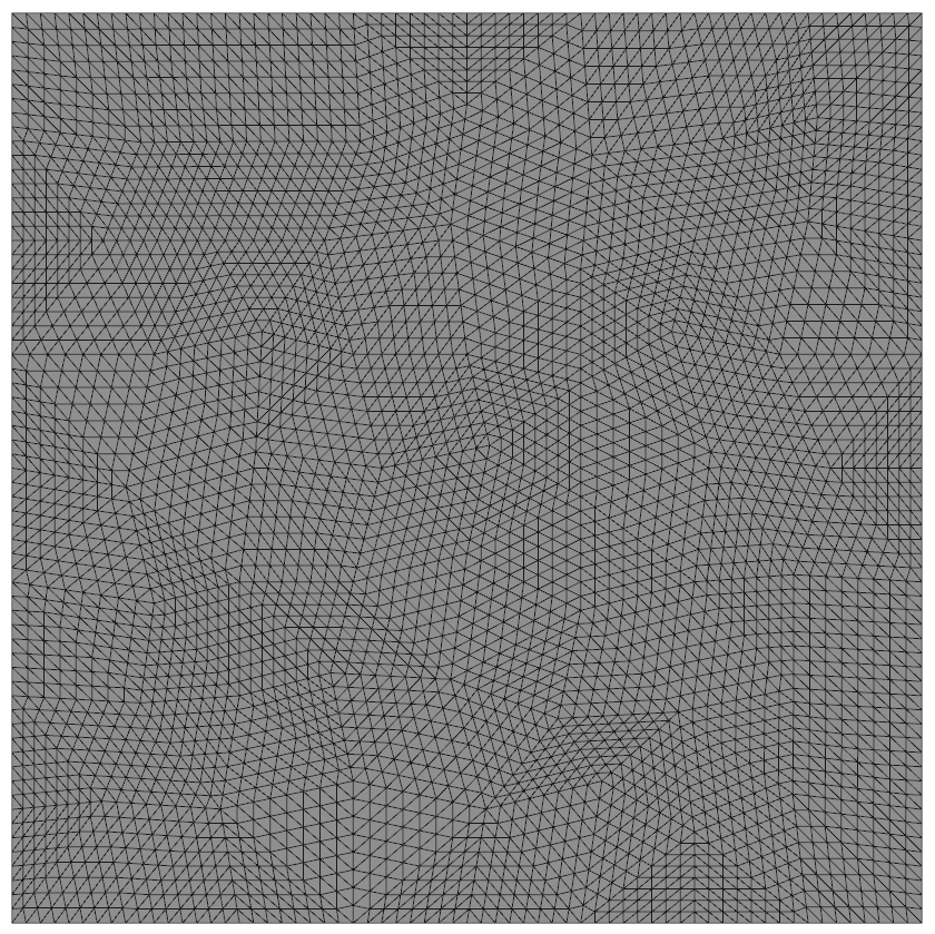
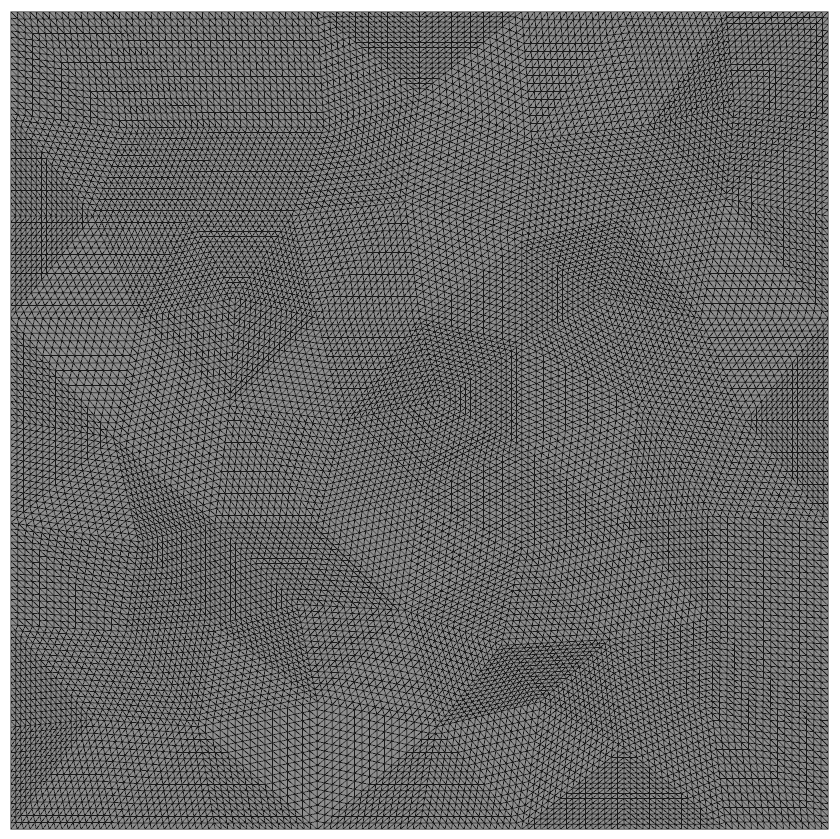
Poisson System on 2D Triangle Meshes
Generalized Barycentric Coordinates
- Wachspress Coordinates
- Wachspress, Warren
- Mean Value Coordinates
- Floater, Hormann, Ju, Wicke
- Maximum Entropy Coordinates
- Sukumar, Hormann
- Harmonic Coordinates
- Joshi, Martin
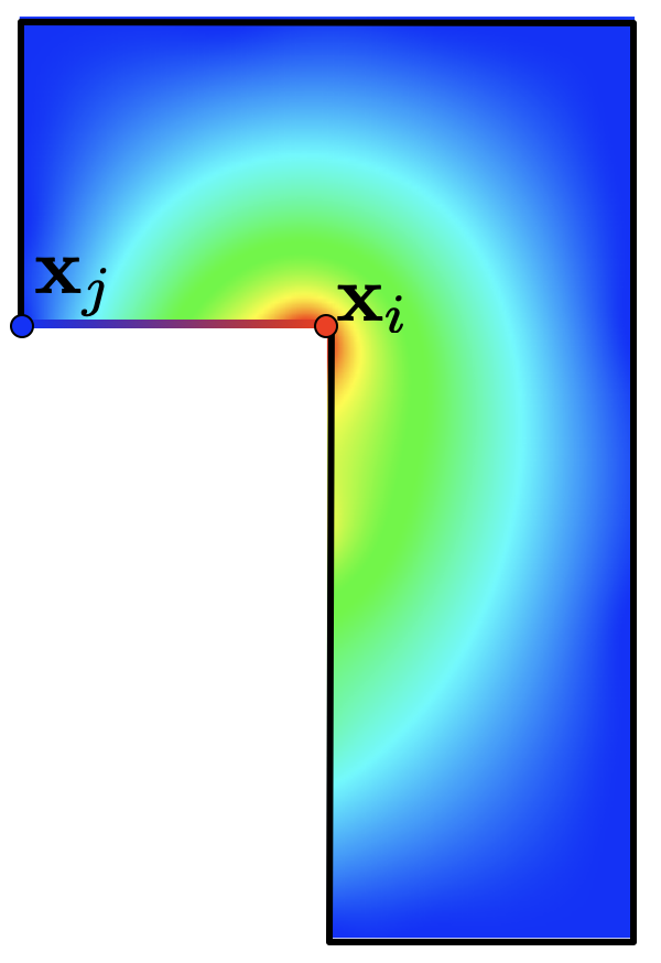
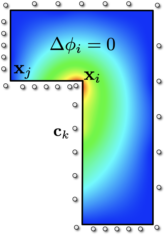
Harmonic Coordinates
- Definition
- Interpolate nodal data: \(\varphi_i(\vec{x}_j) = \delta_{ij}\)
- Linear (=harmonic) on edges
- Harmonic in interior: \(\laplace\varphi_i = 0\)
- Computation
- Method of fundamental solutions
- Approximate shape functions \(\varphi_i\) by RBFs \(\psi_k\) \[\varphi_i(\vec{x}) = \sum_k w_k \, \psi_k\of{\vec{x}} + \pi_1\of{\vec{x}}\]
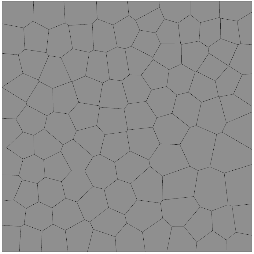
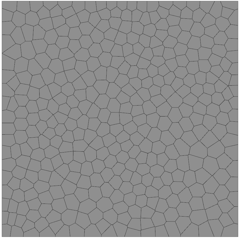
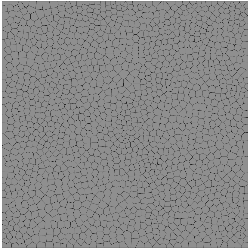
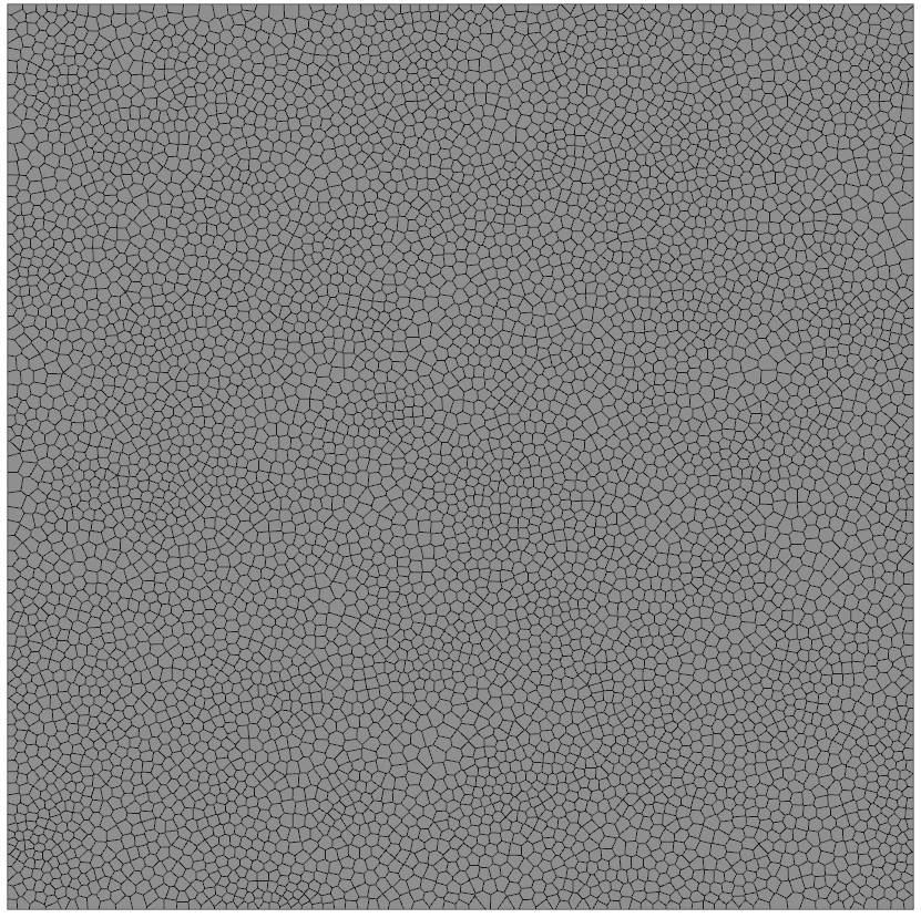
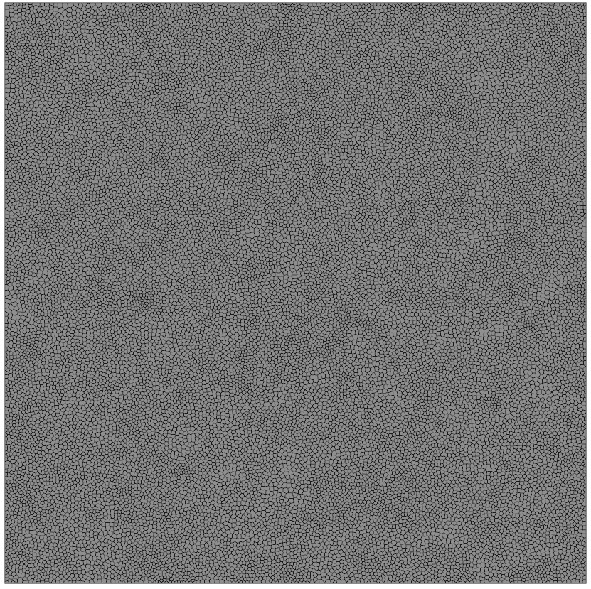
Poisson System on 2D Voronoi Meshes
DEC Polygon Laplacians
- Generalize DEC to non-planar polygons
- Discretization of \(\laplace f = \delta d f\) (Laplace-de Rham)
- The exterior derivative \(d\) becomes the difference operator \(\mat{d}\)
- The co-differential \(\delta\) can be discretized as \(\mat{M}_0^{-1} \mat{d}\T \mat{M}_1\)
- Putting it together: \(\laplace \vec{u} \;\approx\; -\mat{M}_0^{-1} \mat{d}\T \mat{M}_1 \mat{d}\, \vec{u}\)
Difference operator
- The difference operator maps
- From values on vertices (0-forms)

Difference operator
- The difference operator maps
- From values on vertices (0-forms)
- To differece values on (half-)edhes (1-forms)

Strategy I: The algebraic approach

Inner Product Matrix
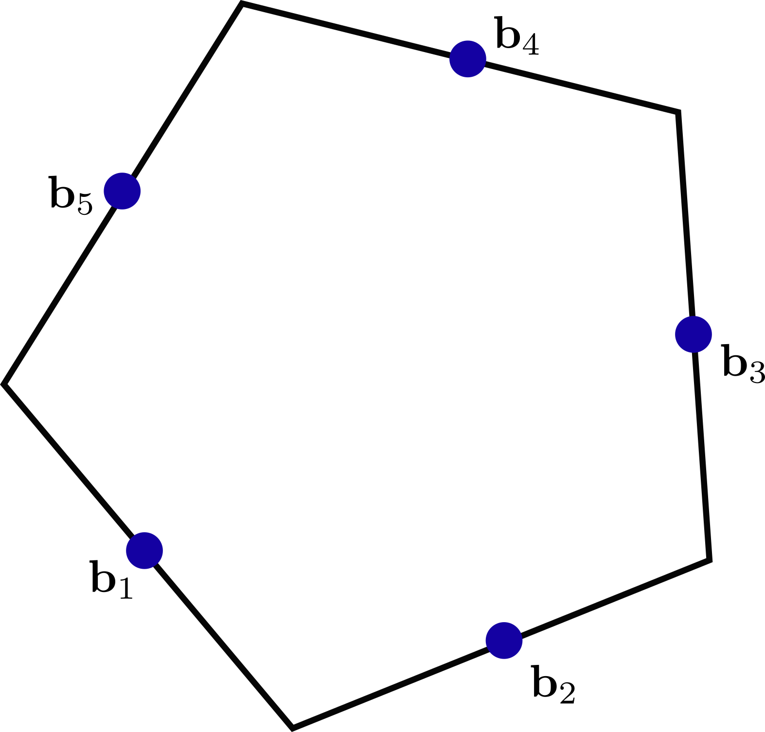
- \(\mat{B}_f = (\vec{b}_1,\dots,\vec{b}_{n_f})^{\mathsf{T}} \in \R^{n_f \times 3}\)
- Rows are barycenters \(\vec{b}_i = \frac{1}{2}\left(\mat{x}_{i+1}+\vec{x}_i\right)\) of each edge \(\vec{e}_i\).
- $|f| $ is vector area of polygon \(f\)
- Define local inner product matrix for 1-forms \[\mat{\tilde{M}}_f = \frac{1}{|f|}\mat{B}_f \mat{B}_f ^{\mathsf{T}}\]
- Not intuitive / easy to see, but not difficult to prove: \[ \grad_{\vec{x}_i}\abs{f} = \left(\tilde{\mat{L}}_f \mat{X}_f\right)_i \]
- Where \(\tilde{\mat{L}}_f = \mat{d}_f \mat{\tilde{M}}_f \mat{d}\)
Fill up the Kernel
- \(\mat{E}_f = (\vec{e}_1,\dots,\vec{e}_{n_f})^{\mathsf{T}} \in \R^{n_f \times 3}\)
- Rows are edge vectors of polygon \(f\).

- Rows are edge vectors of polygon \(f\).
- \(\mathbf{E}_f\T\) has maximal rank 3
- \(\mat{E}_{\bar{f}} = (\bar{\vec{e}}_1,\dots,\bar{\vec{e}}_{n_f})^{\mathsf{T}} \in \R^{n_f \times 3}\)
- Rows are edge vectors of maximal projection \(\bar{f}\).

- Rows are edge vectors of maximal projection \(\bar{f}\).
- \(\mat{E}\T_{\bar{f}}\) has rank 2 \(\rightarrow\) non-trivial kernel
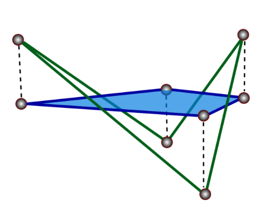
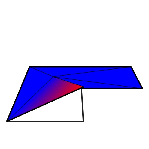
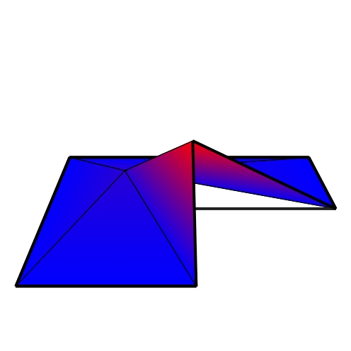
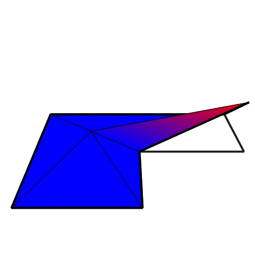
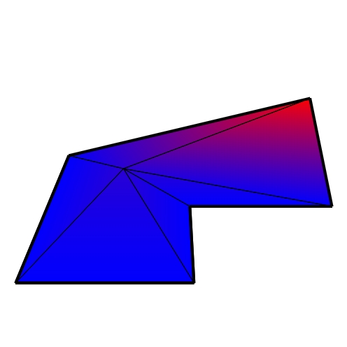
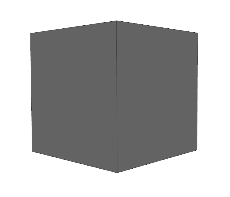
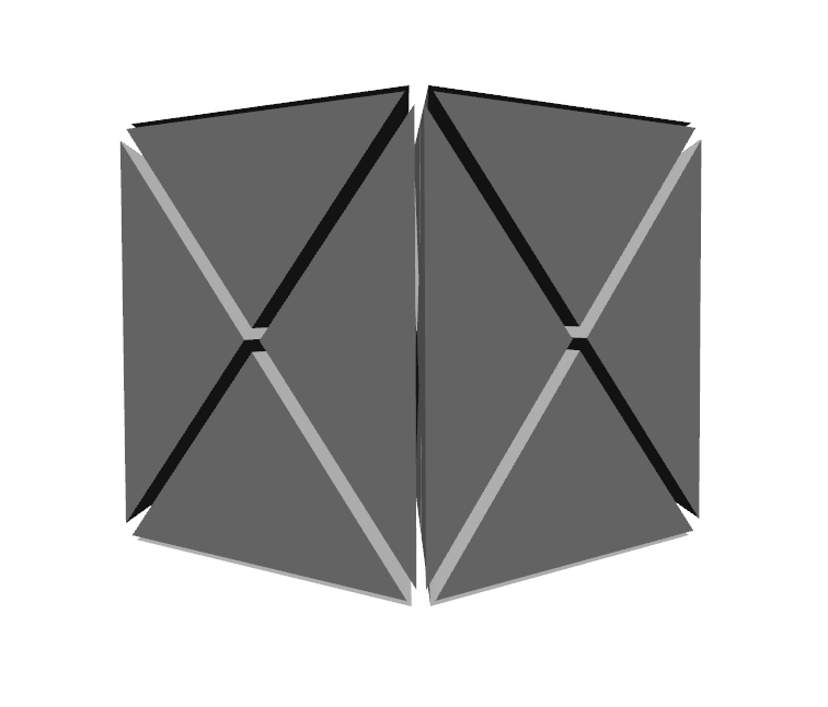
Virtual Simplicial Refinement


Prolongation Operator
\[ {\Huge \downarrow} \; \mat{P} \]
- Insert virtual vertex as affine combination \[ \small \matrix{ \sum_i w_i \vec{x}_{i}\\ \vec{x}_{1}\\ \vec{x}_{2}\\ \vec{x}_{3}\\ \vec{x}_{4}\\ \vec{x}_{5}\\ \vec{x}_{6} } = \underbrace{ \matrix{ w_1 & w_2 & w_3 & w_4 & w_5 & w_6\\ 1 & & & & & \\ & 1 & & & & \\ & & 1 & & & \\ & & & 1 & & \\ & & & & 1 & \\ & & & & & 1 } }_{\mat{P}} \matrix{ \vec{x}_{1}\\ \vec{x}_{2}\\ \vec{x}_{3}\\ \vec{x}_{4}\\ \vec{x}_{5}\\ \vec{x}_{6} } \]
Restriction Operator
\[ {\Huge \uparrow} \; \mat{R} = \mat{P}\T \]
- Redistribute values back to original nodes \[ \mat{R} = \mat{P}\T \]
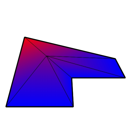
Polygon Shape Functions
\[\downarrow\] \[\downarrow\]
- Insert center vertex through prolongation weights
- Compute standard linear shape functions \(\psi_j(\vec{x})\) on refined polygon
- Coarse shape function for polygon \((\vec{x}_1, \dots, \vec{x}_n)\) with virtual vertex \(\vec{x}_0\) become \[ \varphi_i(\vec{x}) = \psi_i(\vec{x}) + w_i\psi_0(\vec{x}) \,,\quad i \in \{1, \dots, n\} \]
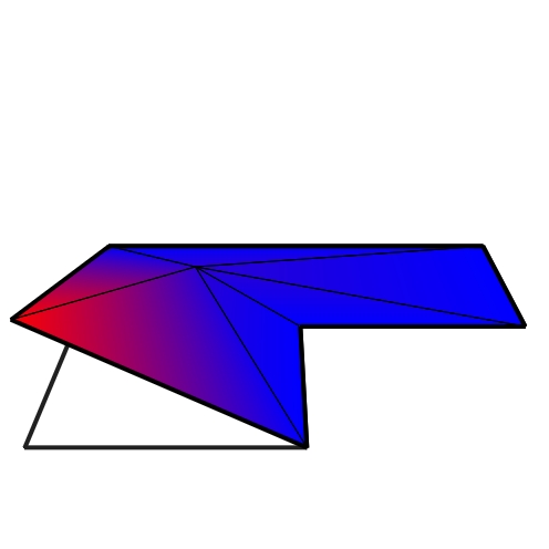
Polygon Shape Functions
- Piecewise linear functions
- Interpolate nodal data: \(\varphi_i\of{\vec{x}_j} = \delta_{ij}\)
- Partition of unity: \(\sum_i \varphi_i\of{\vec{x}} = 1\)
- Barycentric property: \(\sum_i \varphi_i\of{\vec{x}} \vec{x}_i = \vec{x}\)
- \(C^0\) across elements, not \(C^1\) within elements
Choice of Virtual Vertex


Solve linear system for affine prolongation weights 👍
Laplace Matrix & Mass Matrix
- “Sandwiched” Laplace matrix for polygons \[\mat{L} = \mat{P}\T \, \mat{L}^\func{tri} \, \mat{P} \]
- “Sandwiched” mass matrix for polygons \[\mat{M} = \mat{P}\T \, \mat{M}^\func{tri} \, \mat{P} \]
- Laplacian can be factored into divergence and gradient \[ \mat{L} = \underbrace{\mat{P}\T \mat{D}^\func{tri}}_{\mat{D}} \cdot \underbrace{\mat{G}^\func{tri} \mat{P}}_{\mat{G}} \]
Virtual refinement is completely hidden in matrix assembly step!
Linear Shape Functions for Polyhedra

- Insert virtual face point
- Minimizer of squared triangle areas
- Insert virtual cell point
- Minimizer of squared tetrahedra volumes
- Two-step prolongation \[ \mathbf{P} = \mat{P}_c \, \mat{P}_f\]
Discrete Duality Finite Volumes (DDFV)


Quiz
How do we get diamond cells on an arbitrary polygon mesh?
- Subdivide into triangles
- Subdivide into quads
- Connect primal and dual vertices
- Introduce third control mesh


2D DDFV
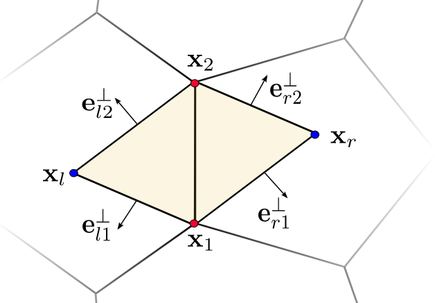
\[ \grad u|_D \;=\; \frac{1}{2 \abs{D}} \sum_{(i,j) \in \partial D} \vec{e}_{ij}^\perp \frac{u_i+u_j}{2} \]
Virtual Dual Vertices
\[\downarrow\] \[\downarrow\]
- Combine ideas from DDFV and virtual refinement
- Use virtual vertices as dual mesh
- Compute DDFV operator on the “virtual diamonds”
- Express diamond in an intrinsic 2D coordinate system
- Restrict values back to the original mesh
Diamond Laplace on Polyhedral Meshes

- Same two-step prolongation as linear virtual refinement method \[ \mathbf{P} = \mat{P}_c \, \mat{P}_f\]
- Construct minimal diamond cells
Volume Diamond Gradient

Linear Elasticity
Locking due to high Poisson ratio 😢
Linear vs Quadratic


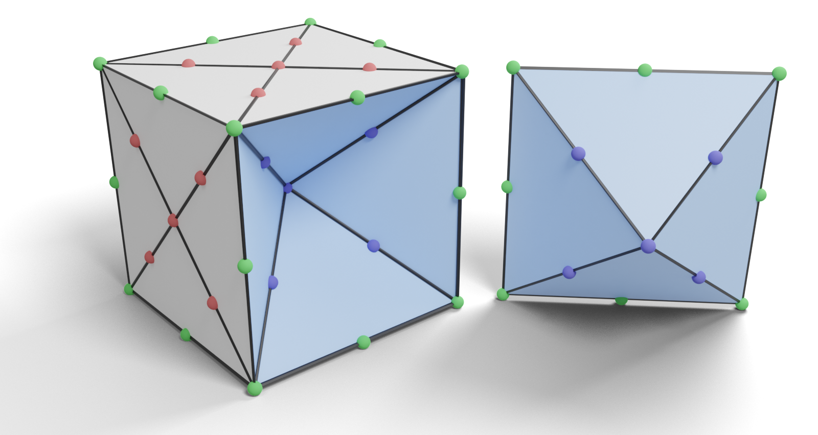
Quiz
Given a quad, how many virtual degrees of freedom do we need for the quadratic Lagrange elements?
- Four virtual vertices
- Five virtual vertices
- Twelve virtual vertices
- Thirteen virtual vertices
Quiz
Given a quad, how many virtual degrees of freedom do we need for the quadratic Lagrange elements?

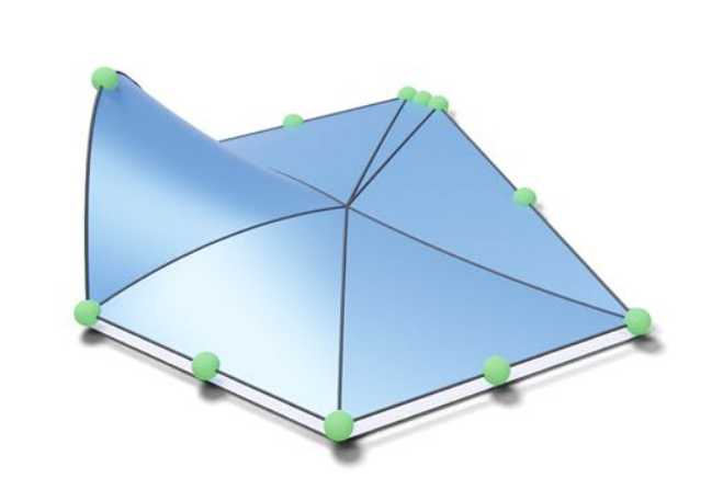
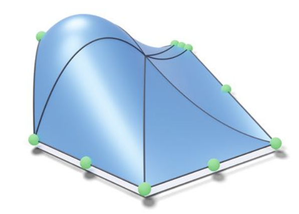
Quadratic Polygon Shape Functions
- Compute standard quadratic shape functions \(\psi_j(\vec{x})\) on refined polygon
- Shape functions for polygon \((\vec{x}_1, \dots, \vec{x}_n)\) with coarse DoFs \(\mathcal{C}\) and virtual DoFs \(\mathcal{K}\) \[ {\color{green}\varphi_i(\vec{x})} = {\color{green}\psi_i(\vec{x})} + \sum_{j\in \mathcal K} w_{ij} {\color{red} \psi_j(\vec{x})} \quad\text{ for } i \in \mathcal C. \]

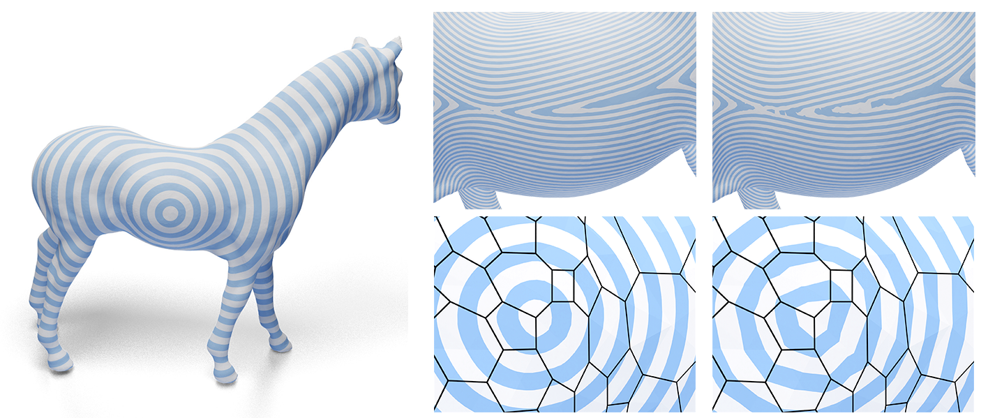
Prolongation Weights Influence Convergence
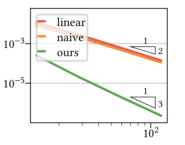
Optimize for Smoothness
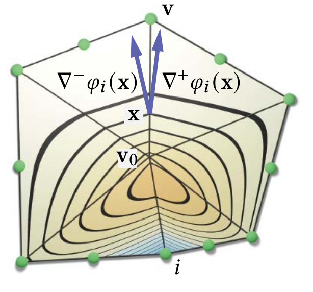
- Shape functions for polygon \((\vec{x}_1, \dots, \vec{x}_n)\) \[ {\color{green}\varphi_i(\vec{x})} = {\color{green}\psi_i(\vec{x})} + \sum_{j\in \mathcal K} w_{ij} {\color{red} \psi_j(\vec{x})} \quad\text{ for } i \in \mathcal C. \]
- Solve variational optimization per cell \[ \min_{\{w_{ij}\}} \sum_{i \in \mathcal C} \sum_{\sigma \in \mathcal E^*} \int_\sigma \norm{ \nabla_\sigma^+ \varphi_i - \nabla_\sigma^- \varphi_i }^2 \ \mathrm{d}\sigma \]
- Only needs a linear system solve 👍
Linear Elasticity
Geodesic Distances
Quadratic Shape Functions for Polyhedra
\[ \small \min_{\{w_{ij}\}} \sum_{i \in \mathcal C} \sum_{\sigma \in \mathcal T^*} \int_\sigma \norm{\nabla_\sigma^+ \varphi_i - \nabla_\sigma^- \varphi_i}^2 \mathrm{d}\sigma \]
Quadratic Shape Functions for Polyhedra
Linear Elasticity
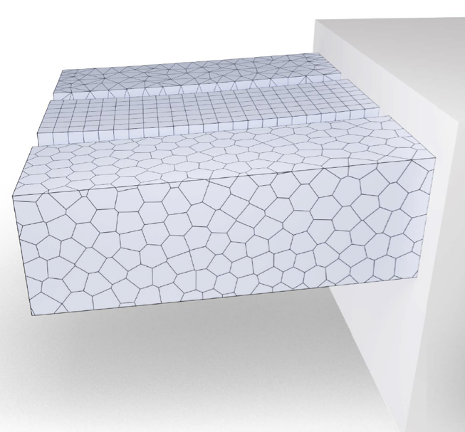
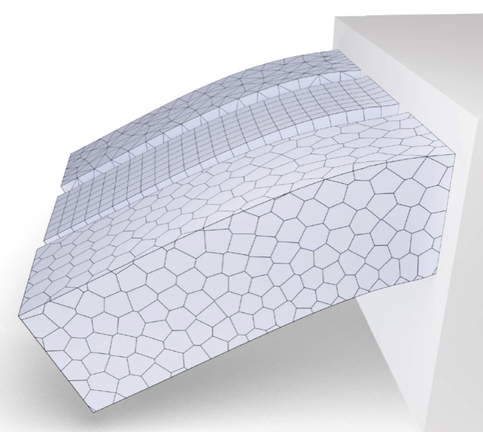
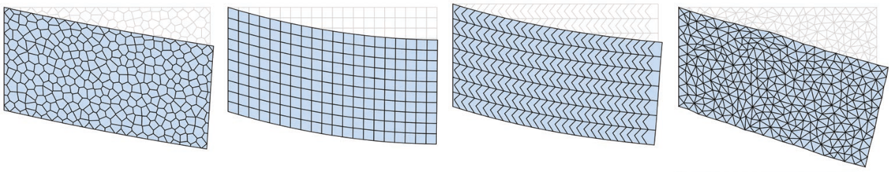
Poisson System on 2D Planes

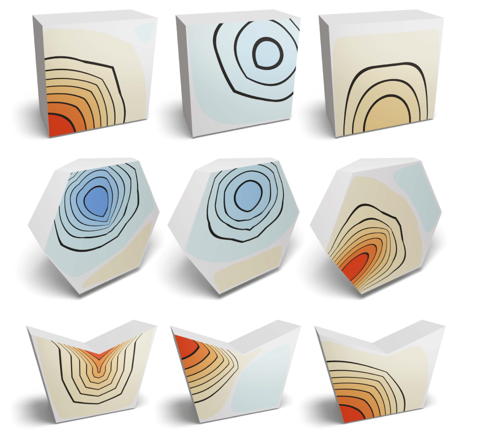
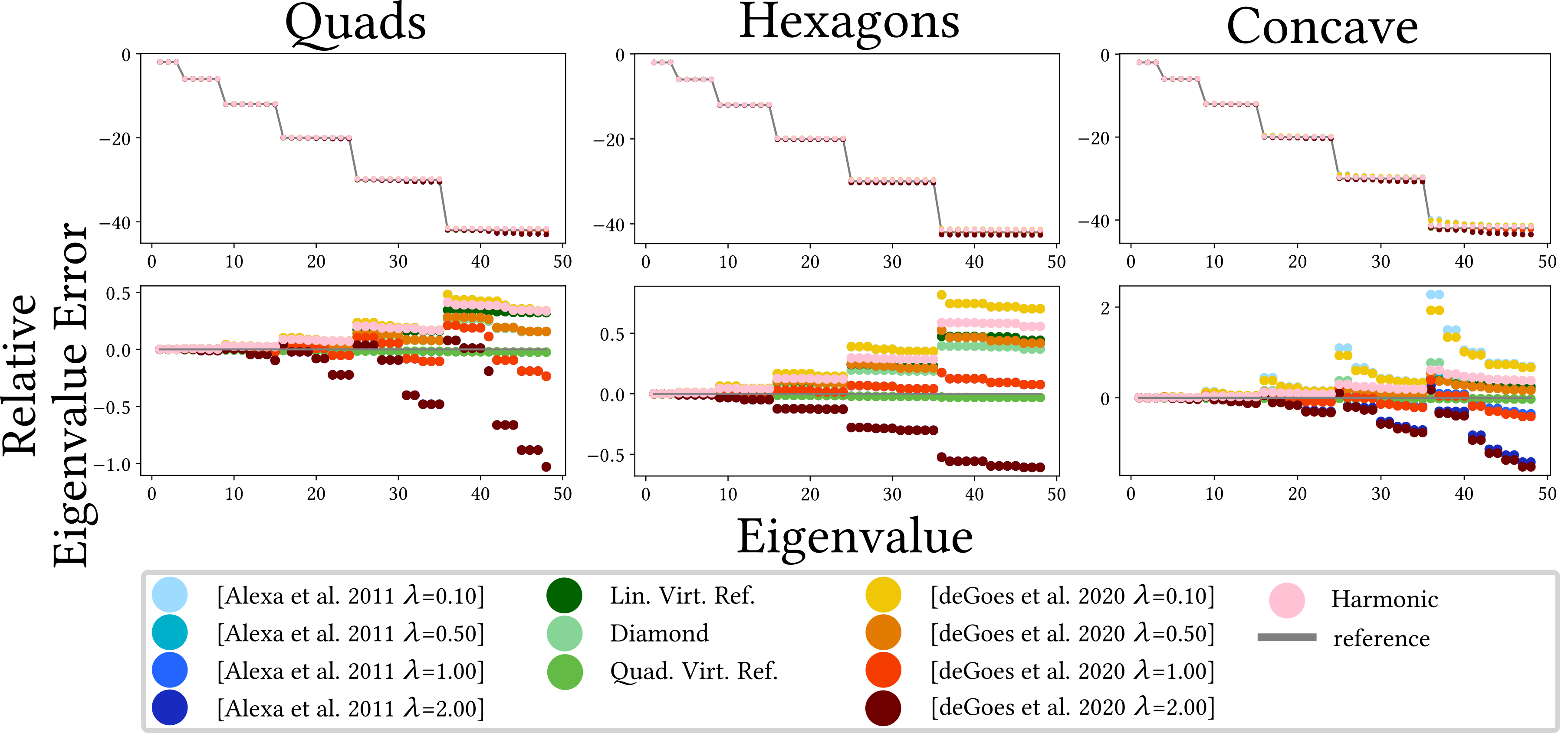
Eigenvalues on Unit Spheres
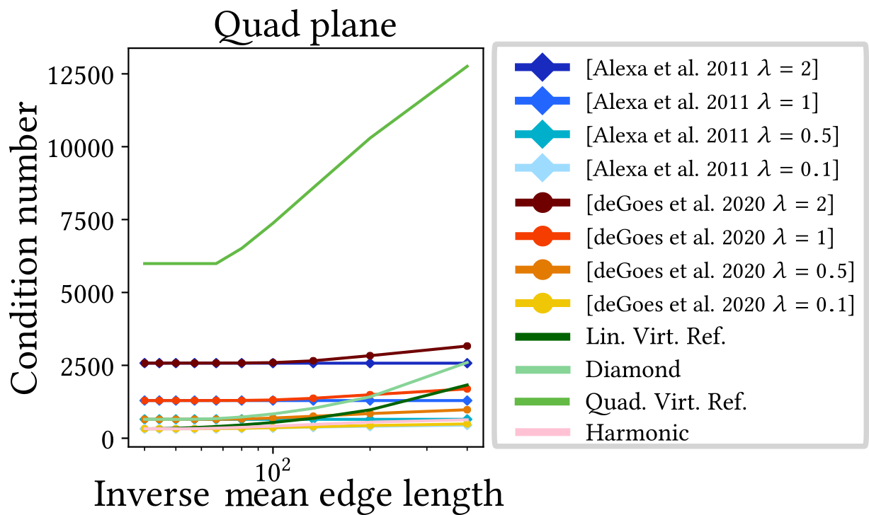
Condition Number
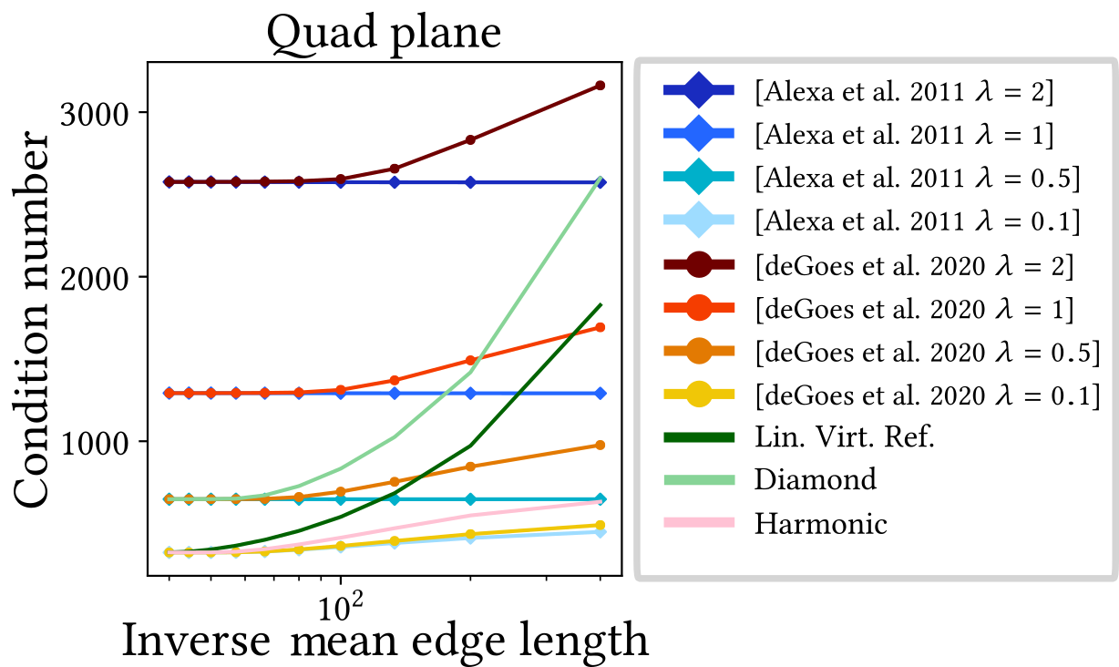
Condition Number
Computational Performance

Computational Performance

Conclusion
- Presented recent progress for Polygon Laplacians
- Discuss individual discretization strategies
- Point out similarities and differences
- Analyze individual strength and weaknesses
- Extensions
- More details on volume meshes (see course notes)

- Acknowledgments
- Collaborators: Philipp Herholz, Misha Kazhdan, Olga Sorkine-Hornung
- Code-Checkers: Fernando de Goes, Max Wardetzky