Sven D. Wagner1, Astrid Bunge2, and Mario Botsch1,3
1TU Dortmund University, Germany
2AutoForm Engineering, Germany
3Lamarr Institute for Machine Learning and Artificial Intelligence, Germany
Abstract
Many applications in geometry processing involve the solution of partial differential equations on discrete surface meshes, with the Laplacian undoubtedly being the most ubiquitous operator in this context. Having discrete operators for gradient, divergence, and Laplacian at hand allows to solve many interesting geometry processing problems.
Introduction
The discrete Laplace-Beltrami operator, or Laplacian for short, is a ubiquitous tool in geometry processing. It allows us to solve numerous partial differential equations on discrete surface meshes, which is essential for various computer graphics applications, like mesh smoothing, mesh parameterization or fairing, followed by many others. For triangulated surfaces, the discrete Laplacian based on the cotangent formula [17, 23, 27, 54, 58] is omnipresent in graphics and geometry processing.
However, despite its seemingly harmless definition (see Equations \(\eqref{eq:triangle_stiffness_matrix}\) and \(\eqref{eq:cotan_weight}\)), there are some factors that need to be considered with regard to the robustness of the cotangent Laplacian. As soon as meshes start to appear in a more degenerate form, numerical stability can become a significant challenge. At the same time, the growing demand for unsupervised processing of large-scale datasets makes the use of efficient and robust implementations of discrete operators more important than ever. Therefore, this course will follow the investigation of Wagner and Botsch [73] and analyze the cotangent implementation of modern general-purpose geometry processing libraries and their resilience to challenging tessellations. Furthermore, we will discuss approaches that go beyond linear FEM and review alternative, more robust Laplace discretizations [8, 60, 65, 73].
Additionally, due to the growing needs in modeling and engineering applications, recent papers point out that the restriction to triangle meshes, while simple and convenient, is no longer sufficient. Many users have to fall back to more general shapes to be able to express geometric properties and features in their model. Applications benefiting from a more flexible range of elements are, for example, fracture modeling [7, 57, 70] or linear elasticity problems [69]. Additionally, since micro-structures of naturally occurring materials like bones can be described through polygonal domains, generalized differential operators are useful tools for the solid- and bio-mechanics community [69]. Furthermore, modeling artists predominantly use quad meshes.
In order to enable this flexibility, several papers within the graphics community developed strategies to generalize the Laplace-Beltrami operator to general polygon meshes. This presents several challenges. For instance, arbitrary polygons might not be inherently planar, potentially resulting in twisted surfaces in 3D. Coming from various backgrounds and inspirations, all introduced Laplacians address these difficulties in their own unique way, but it is not necessarily clear in which aspects the operators actually differ and what their various nuances imply. This tutorial, based on the state-of-the-art report by Bunge and Botsch [17] and course by Bunge et al. [13], therefore intends to showcase occurring similarities between the presented methods that may not be apparent if considered individually.
However, the scope of this course is not limited to the Laplacian operator alone. In the smooth setting, the Laplacian of a function \(f\) is defined as \[ \laplace f = \div \grad f. \] Given their close relation, comparing suitable generalizations for discrete gradient and divergence is an almost equally essential affair focused on in this tutorial. In general, the papers we are going to discuss have all been inspired by different well-known numerical schemes commonly used for various discretization problems. Namely, the Finite Element Method (FEM), the Mimetic Finite Difference Method (MFD), and the Finite Volume Method (FV). Since all generalized Laplacians can be loosely sorted into one of these schemes, we will briefly explain their core principles at the beginning of each section and highlight the inspirational elements that influenced the respective papers.
We start by discussing the required properties a discrete Laplacian should fulfill based on the work presented by Wardetzky et al. [75]. Afterwards, we derive the cotangent Laplacian on standard triangle meshes and examine its numerical stability, followed by a discussion of more robust Laplace discretizations as presented by Wagner and Botsch [73]. We then extend the setting to polygonal meshes, introducing the necessary definitions required for constructing the corresponding operators. Building on this foundation, we provide a more detailed analysis of the involved polygonal operators, their different ideas, and the properties they fulfill. Finally, the different discretizations are evaluated in a variety of quantitative comparisons that address recurring debates within the original papers. In the end, the tutorial intends to provide the reader with an intuition to choose the optimal operator discretization for their given situation.
Basic Definitions
Consider a 2D polygon mesh \(\mathcal{M}=(\mathcal{V},\mathcal{E}, \mathcal{F})\) embedded in 3D, with vertices \(\mathcal{V}\), edges \(\mathcal{E}\), and faces \(\mathcal{F}\). Each vertex \(v_i \in \mathcal{V}\) has an associated 3D position \(\vec{x}_i = (x_i,y_i,z_i)\) and each face \(f\) consists of \(n_f\) vertices. We define an additional set of oriented halfedges \(\mathcal{H}\), where for each inner edge \(e \in \E\) there exist two oppositely oriented halfedges, while each boundary edge has only one.
We define a discrete Laplace operator \(\mathbb{L} \in \R^{\abs{\mathcal{V}} \times \abs{\mathcal{V}}}\) as the product of the inverse of a so-called mass matrix \(\mv{M}\in \R^{\abs{\mathcal{V}} \times \abs{\mathcal{V}}}\) and stiffness matrix \(\mv{L}\in \R^{\abs{\mathcal{V}} \times \abs{\mathcal{V}}}\): \[\begin{align} \mathbb{L} = \mv{M}^{-1}\mv{L}. \end{align}\] \(\mathbb{L}\) is generally referred to as the strong form of the Laplacian and \(\mv{L}\) is its integrated weak form. The exact conditions that are imposed on these matrices will be discussed in the next section. As for their construction, most of the upcoming methods focus on a local approach that builds the required matrices per face. We therefore define:
The matrix \(\mv{X} \in \R^{\abs{\mathcal{V}} \times 3}\) encodes the vertex positions of the mesh in its rows.
\(\mv{X}_f = (\mv{x}^f_1,\dots,\mv{x}^f_{n_f})\tp\) is the \(n_f \times 3\) matrix containing in its rows the cyclically ordered vertex positions \(\mv{x}^f_i\) of the face \(f\).
\(\mv{E}_f = (\mv{e}^f_1,\dots,\mv{e}^f_{n_f})\tp\) is the \(n_f \times 3\) matrix containing in its rows the cyclically ordered edge vectors \(\mv{e}^f_i = \mv{x}^f_{i+1}-\mv{x}^f_i\) of the face \(f\).
\(\mv{B}_f = (\mv{b}^f_1,\dots,\mv{b}^f_{n_f})\tp\) is the \(n_f \times 3\) matrix containing in its rows the barycenters \(\mv{b}^f_i = \frac{1}{2}\left(\mv{x}^f_{i+1}+\mv{x}^f_i\right)\) of each edge \(\mv{e}^f_i\).
Properties of a Discrete General Laplace Operator
The smooth Laplace-Beltrami operator has a set of key structural properties that each discretization should be able to fulfill. The correlation between these smooth properties and discrete Laplace operators has been discussed intensively for triangle meshes by Wardetzky et al. [75]. However, these requirements equally hold for general polygon meshes and are therefore important criteria for the numerical quality of a discrete Laplacian. Unfortunately, as pointed out by Wardetzky et al., most meshes do not allow for Laplacians to satisfy all discrete properties simultaneously, which coins the second part of their paper “No free lunch”. In this section, we will reintroduce the individual definitions presented by Wardetzky et al. [75] in order to establish characteristics by which the quality of each presented polygon Laplacian operator can be assessed.
In the smooth setting, consider a single connected manifold \(\Omega\), possibly with boundary, that is equipped with a Riemannian metric. We define a function \(u:\Omega \rightarrow \R\) and its discrete equivalent \(\mv{u}\in \R^{\abs{\mathcal{V}}}\), whose entries are the function values of \(u\) sampled at the vertices of the surface mesh \(\mathcal{M}\). The strong Laplacian \(\mathbb{L} \in \R^{\abs{\mathcal{V}} \times \abs{\mathcal{V}}}\) defined on \(\mathcal{M}\) is given as a \(\abs{\mathcal{V}} \times \abs{\mathcal{V}}\) matrix pair \(\left( \mv{M}, \mv{L}\right)\) consisting of a sparse symmetric mass matrix \(\mv{M}\) and the weak form of the Laplacian given by the sparse matrix \(\mv{L}\).
Symmetry.
Given two functions \(u\) and \(v\) that are sufficiently smooth and vanish along the boundary of \(\Omega\), the smooth Laplacian is self-adjoint with respect to the \(L^2\) inner product of these functions, meaning \[\begin{align} \langle\Delta u, v\rangle = \langle u,\Delta v \rangle \end{align}\] with \(\langle u, v\rangle = \int_{\Omega} uv \d{A}\). We therefore request the strong form \(\mathbb{L}\) to be a self-adjoint operator with respect to the inner product induced by the symmetric mass matrix \(\mv{M}\), meaning \[\begin{align} &(\mathbb{L} \mv{u})\tp \mv{M} \mv{v} = \mv{u}\tp \mv{M} (\mathbb{L} \mv{v}) \\ \Leftrightarrow \quad & \mv{u}\tp\mv{L}\tp \mv{v} = \mv{u}\tp \mv{L}\mv{v} \end{align}\] for any \(\mv{u}\) and \(\mv{v}\).
Locality.
The smooth Laplacian of a function \(u\) at a point \(\mv{p}\) should only depend on the values \(u(\mv{q})\) of other points \(\mv{q}\) in an \(\epsilon\)-ball around \(\mv{p}\). This means that the discrete Laplacian should also operate locally in the 1-ring neighborhood of the respective vertex and should not be affected by distant vertices in the mesh.
Linear Precision.
In the smooth setting, given a linear function \(u\) defined on \(\Omega\), the Laplacian of said function has to be zero in planar regions of the manifold. The discrete equivalent is similar: Given a planar mesh \(\mathcal{M}\) and any linear function \(u\), we require the strong version of the Laplacian \(\mathbb{L}\) to satisfy \[\begin{equation} \label{eq:linear_precision1} (\mathbb{L}\mv{u})_i = 0 \end{equation}\] for each inner vertex \(v_i\), where \((\cdot)_i\) denotes the \(i\)-th entry or row of the vector or matrix within the parentheses. Alternatively, we can omit the influence of the mass matrix and require the stiffness matrix to satisfy the equivalent condition \[\begin{equation} \label{eq:linear_precision} (\mv{L}\mv{X})_{i} = 0 \end{equation}\] on the vertex positions \(\mv X\).
Positive Semi-Definiteness and Null Space.
In the smooth setting, the Dirichlet energy of a function \(u\) defined on the manifold \(\Omega\) has to be greater than or equal to zero. The discrete version of the Dirichlet energy can be expressed with the help of the stiffness matrix as \[\begin{align} \frac{1}{2}\mv{u}\tp \mv{L} \mv{u}. \end{align}\] Therefore, \(\mv{L}\) has to be positive semi-definite in order for the energy to remain non-negative. Note that, depending on the definition, the Laplacian could alternatively be required to be negative semi-definite. A second aspect of this property addresses the kernel of the Laplacian. The smooth Dirichlet energy vanishes for constant functions. Therefore, the kernel of \(\mv{L}\) has to be one-dimensional as well and can only contain constant functions. If the stiffness matrix can be expressed as \[\begin{align} \label{eq:Kernel_dimension} (\mv{L}\mv{u})_i = \sum_j w_{ij} (u_i - u_j), \end{align}\] the discrete Laplacian automatically fulfills this property [75].
Maximum Principle.
The smooth maximum principle requires that harmonic functions (\(\Delta u = 0\)) have no local extremum at interior points of the manifold \(\Omega\). For example, this property assures that approximated solutions of diffusion problems flow from regions with higher potential to regions with lower potential, instead of the other way round. The discrete equivalent can be directly addressed through the entries of the stiffness matrix by the so-called positive weight property, which is a sufficient but not necessary condition for the discrete maximum principle. It demands that for each vertex \(v_i\) the entries \(\mv{L}_{ij}\) have to be less than or equal to zero if \(i\neq j\) and at least one entry per row has to be nonzero.
Convergence.
The convergence property requires that approximate solutions involving the Laplace operator converge to the exact solution of the PDE under refinement of the mesh, which was analyzed by Hildebrandt et al. [39] and Wardetzky [74]. This property will not be proven for the upcoming operators, but analyzed empirically in the results section.
Laplacians on Triangle Meshes
For triangle meshes, the canonical choice of Laplacian discretization is the cotangent Laplacian. Furthermore, almost all of the later discussed polygon Laplacians reproduce it on triangle meshes. We will therefore revisit its definition based on the finite element discretization, discuss its behavior on (near-)degenerate elements, and describe ways to improve its robustness.
Given a triangle mesh \(\mathcal{M}\), let \(\{\varphi_1, \dots, \varphi_{\abs{\mathcal{V}}} \}\) be the piecewise linear Lagrange basis functions defined on \(\mathcal{M}\), with \[\begin{align}
\label{eq:interpolation_property}
\varphi_i(\mv{x}_j) = \begin{cases}
1 & \text{if } i=j, \\
0 & \text{otherwise.}
\end{cases}
\end{align}\] The mass and stiffness matrices \(\mv{M},\mv{L} \in \R^{\abs{\mathcal{V}} \times \abs{\mathcal{V}}}\) of the Laplace operator are then discretized as \[\begin{equation}
\label{eq:triangle_mass_matrix}
\mv{M}_{ij} = \int_{\mathcal{M}} \varphi_i \cdot \varphi_j = \begin{cases}
\frac{\abs{t_{ijk}}+\abs{t_{jih}}}{12} & \text{if } j \in \mathcal{N}(i), \\
\sum_{k \in \mathcal{N}(i) } \mv{M}_{ik}& \text{if } j =i, \\
0 & \text{otherwise,} \\
\end{cases}
\end{equation}\] and \[\begin{equation}
\label{eq:triangle_stiffness_matrix}
\mv{L}_{ij} = \int_{\mathcal{M}} \langle\grad\varphi_i,\grad\varphi_j\rangle = \begin{cases}
-w_{ij} & \text{if } j \in \mathcal{N}(i), \\
\sum_{k \in \mathcal{N}(i) } w_{ik}& \text{if } j =i, \\
0 & \text{otherwise,} \\
\end{cases}
\end{equation}\] with \[\begin{equation}
\label{eq:cotan_weight}
w_{ij}=\frac{\cot{\alpha_{ij}}+\cot{\beta_{ij}}}{2}.
\end{equation}\] Here \(t_{ijk} = (v_i, v_j, v_k)\) and \(t_{jih} = (v_j, v_i, v_h)\) denote the triangles adjacent to the edge \(e_{ij}\) between the vertices \((v_i,v_j)\),  with \(\abs{t_{ijk}}, \abs{t_{jih}}\) describing their respective areas (see inset). The angles \(\alpha_{ij}\) and \(\beta_{ij}\) lie in the opposite corners of the adjacent triangles and \(\mathcal{N}(i)\) denotes the one-ring neighborhood surrounding \(v_i\).
Emulating the smooth setting with the Laplacian being defined as the divergence of the gradient, one can express the gradient operator as a discrete matrix \(\mv{G} \in \R^{3\abs{\F} \times \abs{\mathcal{V}}}\) consisting of local sub-matrices \(\mv{G}_i \in \R^{3 \times 3}\) per triangle \(f_i=t_{jkl}\). Each column of \(\mv{G}_i\) is associated with the gradient of one of the respective vertices. For example, the first column referring to vertex \(v_j\) would be \[\begin{equation} \label{eq:triangle_gradient} \mv{G}_{i}(:,1) = \frac{(\mv{x}_l-\mv{x}_k)^{\bot}}{2\abs{t_{jkl}}}, \end{equation}\] where \(\vec v^\bot\) denotes a counterclockwise rotation of the vector \(\vec v\) by 90° in the triangle plane. The global matrix \(\mv{G}\) is then assembled by placing the respective face gradients at the column entries of the individual vertices \(v_j\) and setting everything else to zero. This can further be used to discretize the divergence as \[\begin{equation} \label{eq:triangle_divergence} \mv{D} = \mv{G}\tp \hat{\mv{M}}, \end{equation}\] with \(\hat{\mv{M}}\in \R^{3\abs{\F} \times 3\abs{\F}}\) being the diagonal mass matrix containing the area of the triangle \(i\) in the three consecutive diagonal entries associated with face \(i\) [9]. The product of \(\mv{D}\) and \(\mv{G}\) gives us the stiffness matrix \(\mv{L}\), which is consistent with the continuous setting, but requires a concrete embedding of the mesh in contrast to the intrinsic formulation of \(\mv{L}\) itself [64].
Properties
Symmetry.
Considering the individual entries of the stiffness matrix defined in Equation \(\eqref{eq:triangle_stiffness_matrix}\), the cotan operator is symmetric by construction.
Positive Semi-Definiteness and Kernel Dimension.
Since \(\mv{L}\) can be considered as the Gramian matrix of the gradients of the linear Lagrange basis functions, it is positive semi-definite by construction. Given that \(\Delta u(\mv{x}_i)\) of a function \(u\) at vertex \(v_i\) can be expressed through the well known cotan formula [23, 51, 58] \[\begin{align} \Delta u(\mv{x}_i) = \frac{1}{2} \sum_{v_j \in \mathcal{N}(v_i)} (\cot\alpha_{ij}+\cot\beta_{ij}) (u(\mv{x}_j)-u(\mv{x}_i)), \end{align}\]the operator satisfies the condition given in Equation \(\eqref{eq:Kernel_dimension}\) and therefore has a one dimensional kernel.
Locality.
By construction, each row \((\mv{L})_i\) associated to vertex \(v_i\) has non-zero entries only in the columns associated to nodes in its immediate one-ring neighborhood.
Linear Precision.
The area gradient of a triangle \(t_{ijk}\) with respect to the vertex \(v_i\) can be expressed as \[\begin{align} \grad_{\mv{x}_i} A = \frac{\cot{\theta_k}}{2}(\mv{x}_i -\mv{x}_j )+\frac{\cot{\theta_j}}{2} (\mv{x}_i -\mv{x}_k ), \end{align}\] with \(\theta_j\) and \(\theta_k\) denoting the angles at the respective vertices \(v_j\),\(v_k\) and \(A = \abs{t_{ijk}}\) the area of the triangle \(t_{ijk}\). The cotan Laplace of the coordinate function \(\mv{x}_i\) at vertex \(v_i\) can therefore be expressed as the sum of area gradients of its adjacent triangles [23], which, if the triangles all lie within the same plane, becomes zero.
Maximum Principle.
This property is in general not satisfied, since the cotangent becomes negative for angles between 90 and 180 degrees, leading to positive entries \(\mv{L}_{ij}\) in the stiffness matrix if the involved angles satisfy \(\alpha_{ij}+\beta_{ij} > \pi\).
Convergence.
The convergence behavior of the cotan Laplace was discussed by Hildebrand et al. [39] and Wardetzky [74]. They point out that pointwise convergence of refined meshes \(\mathcal{M}\) to a smooth surface \(\Omega\) is not sufficient to guarantee convergence for the cotan Laplace. However, if the meshes converge in Hausdorff distance and are normal graphs over \(\Omega\), then the Laplacian converges to its smooth solution.
Computing the Cotangent Laplacian
While calculating the corner angles of the triangles and applying the cotangent is the easiest way to compute the cotangent weights, as defined in Equation \(\eqref{eq:cotan_weight}\), several mathematical identities can make the calculations more performant and numerically stable. This section describes the different ways to calculate the cotangent Laplacian present in modern geometry processing libraries, as detailed by Wagner and Botsch [73].
Trigonometry.
Trigonometry is still the most widely used method of calculation, but there are several different variations. OpenMesh [10], Geogram [48], VCGLib [72], and CinoLib [50] each first calculate the corner angles using the standard cosine identity \[\begin{equation} \alpha_i = \arccos\left(\frac{\langle \vec e_{ij}, \vec e_{ik}\rangle}{\norm{\vec e_{ij}} \cdot \norm{\vec e_{ik}}}\right) \end{equation}\] at vertex \(v_i\) and triangle \(t_{ijk}\), where \(\vec e_{ij} = \vec x_j - \vec x_i\) is the edge vector from vertex \(v_i\) to \(v_j\). Following this, there exist several variants to compute the cotangent using this angle. For instance, OpenMesh and Geogram compute the cotangent as \(\cot \alpha_i = 1/\tan \alpha_i\), while VCGLib uses the equivalent expression \(\cot \alpha_i = \cos \alpha_i / \sin \alpha_i\). CinoLib, on the other hand, computes the cotangent via the identity \(\cot \alpha_i = \tan(\pi/2 - \alpha_i)\).
Extrinsic Computation.
Expanding the definitions of the trigonometric functions to vector calculus leads to \[\begin{equation} \label{eq:extrinsic} \cot\alpha_i = \frac{\langle \vec e_{ij}, \vec e_{ik}\rangle}{\norm {\vec e_{ij} \times \vec e_{ik}}}, \end{equation}\] which is the definition used by CGAL [71] and geometry-central [63] to calculate the cotangent weights.
Intrinsic Computation.
As the cotangent Laplacian is an intrinsic operator, only depending on edge lengths and connectivity, the above equation can also be rewritten further: \[\begin{align} \langle \vec e_{ij}, \vec e_{ik}\rangle &= \frac{a^2 + b^2 - c^2}{2}, \label{eq:intrinsic}\\ \norm {\vec e_{ij} \times \vec e_{ik}} &= 2|t_{ijk}| = 2\sqrt{s\cdot(s-a)\cdot(s-b)\cdot(s-c)}, \label{eq:heron} \end{align}\] with \(a = \norm{\vec e_{ij}}\), \(b = \norm{\vec e_{ik}}\), \(c = \norm{\vec e_{jk}}\), and \(s = \frac{a+b+c}{2}\). This computation is used by PMP [67], libigl [42], and by geometry-central [63] when explicitly using intrinsic meshes. To improve the numerical stability of the area computation, libigl further uses a sorted variant of Heron’s formula (see Equation \(\eqref{eq:heron}\)), such that \(a \geq b \geq c\) [45].
Clamping.
Although most libraries do not clamp any weights, several options exist to remove unwanted entries from the stiffness matrix. CGAL and PMP ignore cotangent computations whenever the area of the corresponding triangle is zero to avoid dividing by zero. This improves stability in the case of truly degenerate faces. In addition, PMP and CinoLib implement another approach, the clamping of negative weights, which is a sufficient condition to guarantee the maximum principle, but might result in the violation of other properties (e.g., linear precision) [75]. While PMP provides this optionally and per matrix entry, CinoLib clamps each cotangent computation to \(10^{-10}\), thus resulting in a more conservative and less correct result.
Robustness of Implementations.
Wagner and Botsch [73] show in their evaluation that not all implementations offer the same amount of robustness to (near-)degenerate geometry. They recommend avoiding trigonometric computations, as they are by far the least robust due to explicitly and non-robustly computing the corner angles. In their tests, extrinsic computations performed better on meshes with many large angles, while intrinsic computations performed better on tessellations with many small angles and mixed unstructured meshes. Overall, there was no clear winner between the extrinsic and intrinsic approaches, but the trigonometric implementations were the clear losers. Furthermore, they recommend avoiding clamping of negative weights, while ignoring (near-)zero-area triangles can be advantageous.
However, all implementations suffer from problems caused by the overall discretization scheme, leading to many failures and high errors. Investigating the numerical properties of the cotangent Laplacian has been a key research interest, with several works proposing error bounds, quality measures [66, 68], and angle conditions [4, 80] to estimate errors based on the shape of the underlying triangles. Generally, triangles with small angles (needles), large angles (caps), and very small areas (see Figure 2) should be avoided, as they are related to stiffness matrix conditioning, gradient error convergence [66], and ensuring the maximum principle [75].
Robust Laplacians on Triangle Meshes
To improve the robustness of the regular cotangent Laplacian, several modifications have been proposed, related to improving the underlying triangulation [8, 65] or making the Laplacian more robust to (near-)degenerate geometry [60, 73].
Intrinsic Delaunay Laplacian
Bobenko and Springborn [8] propose building the cotangent Laplacian on the intrinsic Delaunay triangulation (iDT), which guarantees the maximum principle but sacrifices locality in the process. This triangulation is built by flipping edges between triangles that do not satisfy the local Delaunay condition \(\alpha_{ij} + \beta_{ij} \leq \pi\), which would result in \(w_{ij} < 0\). However, instead of explicitly flipping the edge, which would result in changed geometry due to the linear nature of extrinsic edges, the edges are represented intrinsically, i.e., via edge lengths. For an intrinsic edge flip, the new edge lengths are instead calculated to preserve the original geometry, resulting in piecewise linear edges. Based on these edge lengths, the cotangent Laplacian can be built using Equations \(\eqref{eq:intrinsic}\) and \(\eqref{eq:heron}\). While this formulation does result in a Laplacian without negative weights \(w_{ij}\), it does not necessarily increase the robustness to (near-)degenerate geometry, as triangles satisfying the local Delaunay condition do not have to be well-shaped.
To improve upon this, Sharp and Crane [65] propose an intrinsic mollification strategy, which increases the length of every edge by a small amount \(\varepsilon > 0\) such that the triangle inequality holds with significant inequality, i.e., \[\begin{equation} \norm{\vec e_{ij}} + \norm{\vec e_{ik}} > \norm{\vec e_{jk}} + \delta \end{equation}\] for all the corners of triangle \(t_{ijk}\) and user-defined tolerance \(\delta > 0\). As such, they choose \[\begin{equation} \varepsilon = \max_{ijk} \max\left(0, \delta-\norm{\vec e_{ij}} - \norm{\vec e_{ik}} + \norm{\vec e_{jk}}\right). \end{equation}\] This improves the intrinsic quality of the mesh, as both caps and needles only barely fulfill the triangle inequality.
Tempered Finite Element Method
The tempered finite element method (TFEM) by Quiriny et al. [60] takes a different approach by altering the discretization scheme itself. They argue that the regular cotangent Laplacian creates a locking phenomenon, where bands of caps that are (nearly) degenerate are only able to interpolate linearly across the band, thus losing the convergence property of the operator. To avoid this, they propose to use a mesh-dependent constant \(C_{\mathcal M} \in \R\) to clamp the Jacobian determinant of the geometric map, which is equal to the double triangle area, e.g., the denominator in Equation \(\eqref{eq:extrinsic}\). This results in the modified computation \[\begin{equation} \frac{\langle \vec e_{ij}, \vec e_{ik}\rangle}{\max \left(\norm {\vec e_{ij} \times \vec e_{ik}}, C_{\mathcal M}\right)}. \end{equation}\] This constant is chosen in relation to the mean edge length \(\bar h\) of the mesh, where the authors propose \(C_{\mathcal M} = C\cdot \bar{h}^3\), with \(C \in \R\) being a mesh-independent constant. While this approach is more resilient to degenerate elements, it does not necessarily fulfill the linear precision property [75], which might be problematic in some applications.
However, Wagner and Botsch [73] argue that this scheme does not result in a scaling-invariant formulation, i.e., the clamping does not only depend on the individual triangle shape. They thus propose some modifications, such as using \(\bar h^2\) instead of \(\bar h^3\) in the definition of \(C_{\mathcal M}\) and using the mean edge length \(\bar h_t\) of the individual triangle \(t \in \mathcal F\) instead of the mean edge length of the mesh. These changes result in their D-TFEM scheme, which only depends on the individual triangle shape, resulting in the modified computation \[\begin{equation} \frac{\langle \vec e_{ij}, \vec e_{ik}\rangle}{\max \left(\norm {\vec e_{ij} \times \vec e_{ik}}, C_{t}\right)} \end{equation}\] with \[\begin{equation} C_t = C \cdot \max\left(\bar h_t, 10^{-10}\right)^2, \end{equation}\] where \(C=10^{-3}\). Furthermore, they also temper the mass matrix, as well as the gradient and divergence, by applying the clamping to the triangle areas in the definitions of \(\mv M\), \(\mv G\), and \(\hat{\mv M}\) described in Section 3.
Comparison of Robust Triangle Laplacians
In their evaluation, Wagner and Botsch [73] show that all alternative Laplacian definitions exhibit significantly increased robustness to (near-)degenerate geometry, even yielding plausible results for meshes with fully-degenerate triangles. However, all approaches except D-TFEM perform notably worse when solving higher-order PDEs, due to the inversion of the mass matrix.
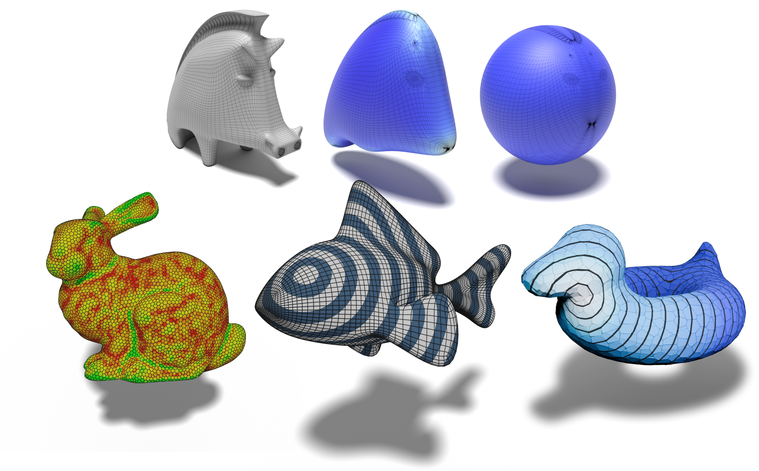
They furthermore investigate the robustness of the other differential operators, i.e., gradient and divergence, when computing geodesic distances using the geodesics in heat approach of Crane et al. [21] (see Section 8.4), as shown in Figure 3. This qualitative comparison shows that the computation can fail for the standard differential operators on real-world examples, such as a mesh generated via VoroMesh [53]. While this also results in artifacts for the exact geodesics computation [55], both the operators based on the mollified iDT and D-TFEM yield stable results.
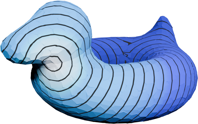
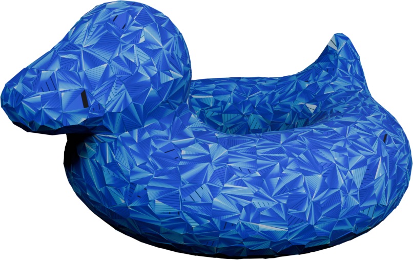
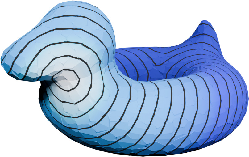
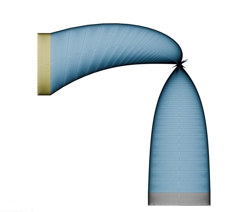
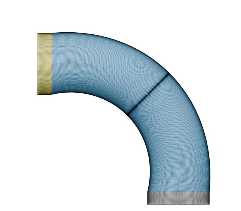
Lastly, because iDT-based operators are inherently intrinsic, they cannot be applied to applications that require extrinsic operators, such as gradient-based editing [78]. However, Wagner and Botsch show that their D-TFEM can also be applied to these use cases involving (near-)degenerate geometry, as seen in Figure 4.
Key Outcomes
In this section, we focused on the standard case of triangle meshes and discussed extensively how to optimize for robustness. There are many ways to compute a discrete Laplacian, and the recommendations of this section can improve results immensely. However, several authors have extended the definition of discrete Laplacians and related operators to more general surface meshes containing arbitrary polygons. These methods and their different mathematical backgrounds will be further explored in the upcoming sections.
Demo: Robustness of Laplacians
When computing geodesic distances or harmonic parameterization for this highly degenerate mesh one observes the D-TFEM Laplacian to yield the most robust results. See the mesh wireframe by changing the drawing mode in the Mesh Info box.
Mimetic Finite Differences
The Mimetic Finite Difference method (MFD) [49] is an approximation strategy whose main goal is to define discrete differential operators that try to preserve, or mimic, certain critical mathematical and physical properties of the underlying PDE. Its core principle lies in the definition of a so-called primary operator, typically gradient, divergence or curl, based on discrete vector and tensor calculus and various forms of Stokes’ theorem. The other operators are then derived by using discrete analogs of Green’s formulas in order to retain a duality relationship to the primary term. Several papers (e.g. [11, 12]) applied the MFD method to derive mimetic discretizations on polygonal and polyhedral meshes and stressed that one of the key components is the definition of an accurate mimetic inner product. This matrix is a vital part in some derivations of the discrete Laplacian. Although the MFD is not directly focused on the construction of this operator, therefore exceeding the scope of this tutorial, its theory influenced recent approaches in the graphics community that will be discussed in the following sections. As a disclaimer, some of the upcoming derivations require rather in-depth knowledge and may seem fast paced for readers that are not already familiar with these terms. However, we still chose to include these detailed explanations in the hope that they might provide some useful insights on the differences of the respective mathematical backgrounds that influenced each of the upcoming discrete polygonal Laplacians.
Mimetic Polygon Laplacian
Alexa and Wardetzky [1] rely on an algebraic approach to define their discrete Laplacian and extend the MFD-based inner product stabilization [11] to two-dimensional manifolds that even allow for non-planar polygons. Given a polygon surface mesh \(\mathcal{M}\) embedded in 3D, the only restrictions are that it has to be oriented, meaning that two adjacent faces have to be oppositely oriented on the shared edge, and that the faces are simple, meaning that they are not self-intersecting and have boundaries that form a closed loop.
Algebraic Framework
Let \(\Gamma^k,\; k\in \{0,1\}\), be the linear function space of discrete \(k\)-forms on \(\mathcal{M}\). A \(k\)-form can be thought of as a function that takes in \(k\)-surfaces and assigns them their integrated value as output, with a 0-surface being a node, a 1-surface an edge, a 2-surface a face, and so on. Alexa and Wardetzky derive their polygon Laplacian for 0-forms from the Laplace-de Rahm operator, which for a scalar-valued function \(u\) is defined as \[\begin{equation} \Delta u = \mathrm{d}^{*}\mathrm{d} u. \end{equation}\] In this context \(\mathrm{d}: \Gamma^0 \rightarrow \Gamma^1\) is the exterior derivative and \(\mathrm{d}^*: \Gamma^1 \rightarrow \Gamma^0\) the codifferential, which is defined as the adjoint of \(\mathrm{d}\) with respect to the square integrable inner product [62]. They use the so-called coboundary operator as a discrete version of the smooth exterior derivative, with \[\begin{align} (\mathrm{d}u)(h_{ij})&= u(j)-u(i) \end{align}\] and \(h_{ij}\) being the oriented halfedge from vertex \(v_i\) to \(v_j\). The definition of a suitable adjoint operator \(\mathrm{d}^{*}\) requires inner products on the \(k\)-form function spaces and is therefore, in contrast to the exterior derivative, metric dependent. The inner products can be expressed as two symmetric positive definite matrices \(\mathbf{M} \in \R^{\abs{\mathcal{V}}\times \abs{\mathcal{V}}}\) and \(\mathbf{M}_1 \in \R^{\abs{\mathcal{H}}\times \abs{\mathcal{H}}}\). Any choice of \(\mathbf{M}\) and \(\mathbf{M}_1\) gives us an expression for the discrete Laplacian \[\begin{align} \mathbb{L} = \mathrm{d}^{*}\mathrm{d} = \mv{M}^{-1}\mv{L} \end{align}\] with \[\begin{align} \mv{L} = \mv{d}\tp \mv{M}_1 \mv{d}. \end{align}\] The matrix version of the coboundary operator \(\mv{d} \in \R^{\abs{\mathcal{H}}\times \abs{\V}}\) is often referred to as the difference operator. Its \(k\)-th row associated with the \(k\)-th halfedge \(h_{ij}\in \mathcal{H}\) can be expressed as \[\begin{align} \label{eq:coboundaryoperator} \mv{d}_{kl} = \begin{cases} -1 & l=i, \\ 1 & l=j,\\ 0 & \text{ otherwise,} \end{cases} \end{align}\] which is only non-zero for the entries \(\mv{d}_{ki}\) and \(\mv{d}_{kj}\) associated with the vertices connected by the halfedge.
Choice Of Inner Product Matrices
Although in theory any choice for the two inner product matrices would be feasible, not all of them yield the same quality of results. Alexa and Wardetzky therefore motivate their chosen construction by fulfilling the desired criteria discussed in Section 2.1. The inner product matrix for 0-forms assigns each vertex a certain mass. In order to retain locality, the matrix \(\mv{M}\) is given by \[\begin{equation} \label{eq:0form_matrix} \mv{M}_{ii} = \sum_{f \ni v_i} \frac{\abs{f}}{n_f}, \end{equation}\] where \(\abs{f}\) denotes the magnitude of the polygons’ vector area. As already mentioned, we also consider non-planar polygons in \(\R^3\) that do not necessarily define a surface. Therefore, \(\abs{f}\) is defined as the area of the largest orthogonal projection of the polygon onto a plane and can be computed as the norm of the Darboux vector \(\mv{a}_f \in \R^3\) of the skew symmetric \((3 \times 3)\) matrix \[\begin{equation} \label{eq:area_matrix} \mv{A}_f = \mv{E}_f\tp \mv{B}_f, \end{equation}\] meaning \[\begin{equation} \label{eq:face_magnitude} \abs{f} = \norm{ \mv{a}_f} = \norm{\frac{1}{2}\sum_{v_i\in f}\mv{x}_{i} \times \mv{x}_{i+1}}. \end{equation}\] The cyclic vertex positions \((\mv{x}_{i} ,\mv{x}_{i+1})\) depend on the orientation of the face, which is encoded in the previously defined matrix \(\mv{X}_f\). It makes sense to look at the definition of the inner product for 1-forms from a local perspective per face and then later assemble the individual matrices into the global representation, since the process can be repeated per element \(f\in \F\). The starting point for the construction is the matrix \(\mv{\tilde{M}}_f \in \R^{n_f \times n_f}\) given by \[\begin{equation} \label{eq:innerProduct_Brezzi} \mv{\tilde{M}}_f = \frac{1}{\abs{f}} \mv{B}_f\mv{B}_f\tp, \end{equation}\] which was previously defined by Brezzi et al. [11] and is motivated by the Laplacian’s connection to mean curvatures. However, while this choice of inner product matrix is generally positive semi-definite, in order for the Laplacian itself to fulfill this property, which is a desired criterion, the inner products have to be positive definite. Alexa and Wardetzky therefore add a stabilization term to extend Brezzi et al.’s definition to non-planar polygons and give rise to a positive definite inner product. The necessity stems from the fact that for general polygons with \(n_f\) vertices the transposed midpoint matrix \(\mv{B}_f\) will have either rank 2 (planar) or 3 (non-planar), allowing for a kernel of dimension \(n_f - \text{rank}(\mv{B}_f)\). Therefore, in order to fill up the kernel, Alexa and Wardetzky introduce the alternative inner product matrix \[\begin{equation} \label{eq:innerProduct_AW} \mv{M}_f := \mv{\tilde{M}}_f + \mv{C}_{\bar{f}} \mv{U}_{\bar{f}} \mv{C}_{\bar{f}}\tp. \end{equation}\] Here, \(\bar{f}\) is the maximum orthogonal projection of the polygon \(f\) and \(\mv{C}_{\bar{f}} \in \R^{n_f \times (n_f-2)}\) is a matrix whose columns span the kernel of \(\mv{E}_{\bar{f}}\tp\). Combined with any choice of a symmetric positive definite matrix \(\mv{U}_{\bar{f}} \in \R^{n_f \times n_f}\), the stabilization term will lead to a positive definite inner product \(\mv{M}_f\), as proven in Theorem 1 of the original paper. That \(\mv{C}_{\bar{f}}\) only has to span the kernel of \(\mv{E}_{\bar{f}}\tp\) is motivated by the linear precision property. In order for \((\mv{L}\mv{X})_i\) to vanish in a planar region surrounding vertex \(v_i\), the stabilization term must also vanish. But since \(\mv{E}_f = \mv{E}_{\bar{f}}\) for planar polygons, we get \[\begin{equation} \label{eq:Alexa_linprecision} \left(\mv{C}_f\tp\mv{d}_f\mv{X}_f\right)_i = \left(\mv{C}_f\tp\mv{E}_f\right)_i = \left(\mv{C}_f\tp\mv{E}_{\bar{f}}\right)_i \stackrel{!}{=} 0, \end{equation}\] which is equivalent to \[\begin{align} \left(\mv{E}_{\bar{f}}\tp\mv{C}_f\right)_i \stackrel{!}{=} 0. \end{align}\] Here, \(\mv{d}_f\) refers to the local difference operator defined on the face \(f\). Since all other properties are already accounted for, it is sufficient to require that \(\mv{C}_f\) spans the kernel of \(\mv{E}_{\bar{f}}\tp\). As for inner products in general, there are several choices for \(\mv{C}_{\bar{f}}\) and \(\mv{U}_{\bar{f}}\) that would satisfy the conditions, giving rise to a whole family of suitable matrices. However, Alexa and Wardetzky propose a special combination in order to achieve scale invariance as a property for the final Laplacian, meaning that the stiffness matrix \(\mv{L}\) remains unchanged when the mesh is uniformly scaled. Using a parameter \(0 < \lambda \in \R\), they choose the matrix \(\mv{U}_{\bar{f}}\) as \[\begin{equation} \mv{U}_{\bar{f}} := \lambda \mv{I}_f, \end{equation}\] with \(\mv{I}_f\) being the \(n_f\)-dimensional identity matrix. They choose \(\mv{C}_{\bar{f}}\) such that its columns are orthonormal, and the final inner product leads to a per-face Laplacian stiffness matrix \[\begin{align} \mv{L}_f = \mv{d}_f \tp \mv{M}_f \mv{d}_f \end{align}\] that is not affected by scaling, is local and linearly precise. These local matrices are then assembled into the global stiffness matrix \(\mv{L}\) by assigning each vertex \(v_i\) the \(i\)-th row and column of \(\mv{L}\) in which the sum over their respective entries in the local matrices are collected.
Geometric Polygon Laplacian
Alexa and Wardetzky’s focus lies solely on the definition of the Laplace-Beltrami and did not further investigate other operators. This was later addressed by de Goes et al. [32], who defined a variety of discrete differential polygon operators that also serve as a generalization of the MFD, but with a stabilization term for the inner product matrix on 1-forms inspired by the virtual element method (VEM) [5]. The following section will further elaborate on their approach. The main focus of de Goes et al. [32] was a new linearly precise discretization of the gradient, which allows to define a consistent set of operators, including their own interpretation of the Laplacian.
Polygon Gradient
As in the previous section, the definition of the gradient will be applied locally per polygon \(f\in\F\), but can be assembled into a global gradient matrix acting on the complete mesh. Given a scalar function \(u\) defined on \(f\), we want to find a matrix \(\mv{G}_f\) that simulates the behavior of the gradient \(\grad u\) on the polygon. For planar elements, this would normally be achieved by applying Stokes’ theorem to \(\grad u\) and deriving a matrix discretization through the weak form of the resulting boundary integral. However, since the polygons of the given mesh are not necessarily planar it is not clear how to define the surface normal \(\mv{n}(\mv{x})\) at the boundary points \(\mv{x}\). Therefore, the standard approach cannot be used. De Goes et al. [32] circumvent this problem by evaluating the co-gradient operator \[\begin{align} \grad u^{\bot}(\mv{x}) := \mv{n}(\mv{x}) \cross \grad u(\mv{x}), \end{align}\] on which applying Stoke’s theorem leads to \[\begin{equation} \label{eq:Cograident_Stokes} \iint_f \grad u^{\bot}(\mv{x}) \d{A} = \oint_{\partial f} u(\mv{x}) \mv{t}(\mv{x}) \d{\mv{x}}, \end{equation}\] with \(\mv{t}(\mv{x})\) being the unit tangent vector at boundary point \(\mv{x}\). This expression is independent of the surface of the polygon and only requires the tangent vectors along the boundary, which are uniquely defined. For example, if we consider the boundary integral in Equation \(\eqref{eq:Cograident_Stokes}\) for linear functions \(u\), the integrated co-gradient can be evaluated exactly as a sum over the averaged function values along the polygon edges, multiplied with the respective edge vector: \[\begin{equation} \oint_{\partial f} u(\mv{x}) \mv{t}(\mv{x}) \d{\mv{x}} = \mv{E}_f\tp \mv{Avg}_f \mv{u}_f. \end{equation}\] Here \(\mv{Avg}_f \in \R^{n_f \times n_f}\) is a matrix that yields the average of consecutive vector entries, defined as \[\begin{align} \left(\mv{Avg}_f\right)_{ij} =\begin{cases} \frac{1}{2} & \text{for } j = i \\ \frac{1}{2} & \text{for } j= (i+1) \text{ mod } n_f \\ 0 &\text{otherwise.} \end{cases}\end{align}\] Additionally, in order to describe the co-gradient as matrix-vector multiplication, one can define the cross product as a map from a 3D vector \(\mv{p}=(p_1,p_2,p_3)\tp\) to a skew symmetric matrix \([\mv{p}] \in \R^{3\times 3}\) with \[\begin{equation} [\mv{p}] = \begin{pmatrix} 0 & -p_3 & p_2 \\ p_3 & 0 & -p_1 \\ -p_2 & p_1 & 0 \\ \end{pmatrix}, \end{equation}\] such that \([\mv{p}]\mv{q} = \mv{p} \times \mv{q}\) for \(\mv{q} \in \R^3\). If we consider \(u: \R^3 \rightarrow \R\) to be a linear function, meaning \(u(\mv{x}) = \mv{s}\tp \mv{x} + r\) with \(\mv{s},\mv{x} \in \R^3\) and \(r\in \R\), its co-gradient would yield \(\mv{n}(\mv{x})\cross \mv{s}\), which can then be expressed as \([\mv{n}(\mv{x})] \mv{s}\). This becomes useful if we consider \[\begin{align} \iint_f \grad u^{\bot}(\mv{x}) \d{\mv{x}} = &\oint_{\partial f} \left(\mv{s}\tp \mv{x} + r \right) \mv{t}(\mv{x}) \d{\mv{x}} \\ = & \mv{E}_f\tp \mv{Avg}_f\left( \mv{X}_f \mv{s} + \mv{1}_fr \right) \\ = & \mv{E}_f\tp\mv{B}_f \mv{s}, \end{align}\] which equally gives \[\begin{equation} \label{eq:normal_integral} \mv{E}_f\tp\mv{B}_f \mv{s} = \left(\iint_{f} [\mv{n}(\mv{x})] \d{\mv{x}} \right) \mv{s}, \end{equation}\] since the term \(\mv{E}_f\tp \mv{Avg}_f\mv{1}_f = \mv{E}_f\tp\mv{1}_f\), which is the sum of edge vectors and therefore zero. Equation \(\eqref{eq:normal_integral}\) implies that the surface integral of the matrix \([\mv{n}(\mv{x})]\) is equal to the previously mentioned area matrix \(\mv{A}_f\) (see Equation \(\eqref{eq:area_matrix}\)) related to the largest orthogonal projection of the face \(f\) and independent of the polygons’ interpolated surface. Therefore, replacing the normal term \(\mv{n}(\mv{x})\) with the constant face normal of the planar projection \(\bar{f}\), given by \[\begin{align} \mv{n}_f = \frac{\mv{a}_f}{\abs{f}}, \end{align}\]the surface integral of the co-gradient can be changed to \[\begin{align} \iint_f [\mv{n}_f] \grad u(\mv{x}) \d{\mv{x}}. \end{align}\] Considering that the co-gradient \(\grad u^{\bot}\) can now be interpreted as a local 90 degrees rotation of the gradient around the normal \(\mv{n}_f\), one can apply a second rotation around the same normal to obtain \(-\grad u\). This leads to de Goes et al.’s definition of the the gradient matrix \[\begin{equation} \label{eq:geometric_gradient} \mv{G}_f = - \frac{1}{\abs{f}} [\mv{n}_f]\mv{E}_f\tp \mv{Avg}_f \end{equation}\] per polygon \(f\), which is proven to be linearly precise. As for the stiffness matrix, the local gradient operators can be assembled into a global gradient operator per mesh \(\mv{G}\in \R^{3 \abs{\F} \times \abs{\mathcal{V}}}\).
Flat, Sharp And Projection Operator
Based on their definition of the gradient operator, de Goes et al. derive an alternative expression to Alexa’s and Wardetzky’s choice for the inner product matrix on 1-forms. Involved in the process are their discrete polygon extensions of the so-called sharp \(\sharp\) and flat \(\flat\) operators, both discretized as \[\begin{equation} \label{eq:sharpOperator} \mv{V}_f^{\sharp}:= \frac{1}{\abs{f}}[\mv{n}_f]\left(\mv{B}_f\tp - \mv{c}_f\mv{1}_f\tp\right) \in \R^{3 \times n_f}, \end{equation}\] and \[\begin{equation} \label{eq:flatOperator} \mv{V}_f^{\flat} := \mv{E}_f \left(\mv{I}-\mv{n}_f\mv{n}_f\tp\right) \in \R^{n_f \times 3} \end{equation}\] respectively, with \(\mv{c}_f\) being the face centroid and \(\mv{1}_f \in \R^{n_f}\) a vector with only ones as entries. As pointed out in Lemma 2 of the original paper, this expression for the sharp operator yields \[\begin{align} \mv{G}_f \mv{u}_f= \mv{V}_f^{\sharp} \mv{d}_f \mv{u}_f, \end{align}\] for any scalar function \(\mv{u}_f\) and is therefore able to reproduce a discrete version of the smooth relation \(\grad u = (\mathrm{d}u)^{\sharp}\) between sharp and gradient operator. In the continuous setting, given a vector space \(V\) equipped with an inner product \(\langle \cdot,\cdot \rangle\) represented by a matrix \(\mv{K}\): \[\begin{align} \langle \mv{x}, \mv{y} \rangle = \mv{x}\tp \mv{K} \; \mv{y} \quad \forall \; \mv{x},\mv{y} \in V, \end{align}\] the flat operator \(\flat\) is defined as \[\begin{equation} \mv{v}^{\flat}(\mv{u}) = \langle \mv{v}, \mv{u} \rangle = \mv{v}\tp \mv{K}\; \mv{u}, \end{equation}\] mapping a vector \(\mv{v}\) from the vector space \(V\) to a functional \(g(\mv{u}) = \langle \mv{v}, \mv{u} \rangle\) in its dual space \(V^*\) [47]. The flat and sharp operators form an isomorphism and we know from the previous assumption that for each linear functional \(g \in \mathcal{V}^*\) there exists a unique \(\mv{v} \in V\) such that \(g(\mv{u}) = \langle \mv{v}, \mv{u} \rangle\) for all \(\mv{u} \in V\). Therefore, the sharp operator \(\sharp\) forms the inverse of \(\flat\) and can be considered as \(g^{\sharp} = \mv{v}\). This is commonly referred to as lowering or raising an index. In de Goes’ setting, the matrix \(\mv{V}^{\flat}\) maps a 3D vector to its tangential part and then computes its counter-clockwise circulation along the edges of the polygon, giving us a discrete 1-form. The sharp operator \(\mv{V}^{\sharp}\) inversely maps the values of a discrete 1-form defined on the polygon back to a single tangent vector per face. However, in contrast to the continuous setting, the operators defined by de Goes et al. are not the exact inverses of each other. The definition holds for any vector \(\mv{v} \in \R^3\) that satisfies \(\mv{v}\tp \mv{n}_f= 0\), meaning it is tangent to the polygon. If this vector is flattened to a 1-form and then inversely sharpened back, it regains its original form. However, first applying the sharpening operator and then lowering the resulting tangent vector back to its 1-form does not have the same effect due to the rank deficiency of \(\mv{V}_f^{\sharp}\). It reduces the \(n_f\) values of a discrete 1-form to only a tangent vector on the polygon \(f\) [32] and therefore loses information. Inspired by the virtual element method [5], they mitigate the effect by defining a so-called projection operator \[\begin{equation} \mv{P}_f := \mv{I}_f - \mv{V}_f^{\flat}\mv{V}_f^{\sharp} \quad \in \R^{n_f \times n_f} \end{equation}\] that measures the error of \(\mv{V}_f^{\flat}\) and \(\mv{V}_f^{\sharp}\) being inverse to each other. Basically, by first sharpening a 1-form \(g\) to a tangent vector that is then flattened back to a representative 1-form \(\hat{g}\), the projection operator eliminates the components of \(g\) that would result in a tangent vector after applying \(\mv{V}_f^{\sharp}\).
Stiffness Matrix
Equipped with the previously defined operators, de Goes et al. [32] define their local inner product matrices acting on 1-forms as \[\begin{equation} \label{eq:innerProduct_dG} \mv{M}_f := \abs{f} \mv{V}_f^{\sharp \mathsf{T}} \mv{V}_f^{\sharp } + \lambda \; \mv{P}_f \tp \mv{P}_f, \end{equation}\] which can be assembled into the global inner product matrix \(\mv{M}_1\) acting on the whole mesh. The matrix \(\mv{M}_f\) maps the involved 1-forms to their respective tangential vectors with the help of the sharpening operator \(\mv{V}_f^{\sharp}\), resulting in their dot product. The potential rank deficiency is mitigated through the second correction term regulated by a parameter \(\lambda >0\). As for Alexa and Wardetzky, this regularization is necessary to guarantee that the inner product matrix is strictly positive definite, which can then be used as before to define the local discrete Laplace-Beltrami operator \[\begin{equation} \mv{L}_f = \mv{d}_f\tp \mv{M}_f \mv{d}_f. \end{equation}\]
Gradient and Divergence Operator
Since the Laplacian of a function \(u\) is defined as the divergence of the gradient of said function \[\begin{equation} \Delta u = \div(\grad u), \end{equation}\] its discretization should be able to simulate the same behavior. This means that for each gradient matrix \(\mv{G}_f \in \R^{3 \times n_f}\) defined on a polygon \(f\), there should exist a respective divergence matrix \(\mv{D}_f \in \R^{n_f \times 3}\) with \[\begin{equation} \label{eq:divergenceGradient} \mv{L}_f = \mv{D}_f \mv{G}_f. \end{equation}\] Typically, this divergence operator is defined as the adjoint of the gradient scaled with a mass matrix containing the faces areas. However, a possibility for both presented approaches [1, 32] to satisfy Equation \(\eqref{eq:divergenceGradient}\) would be to follow the discrete exterior calculus interpretation [22] of the operators. Here, the difference matrix \(\mv{d}_f\) can be seen as a gradient operator acting on \(0\)-forms and the divergence of a discrete 1-form on \(f\) is then defined as \[\begin{equation} \label{eq:geometric_divergence} \mv{D}_f := \mv{d}_f\tp \mv{M}_f, \end{equation}\] which gives the required equality. Note that this interpretation of the gradient differs from de Goes’ geometric operator in Equation \(\eqref{eq:geometric_gradient}\). In fact, given that their sharp operator satisfies \(\mv{V}_f^{\sharp}\mv{d}_f = \mv{G}_f\), we can interpret their \(\mv{L}_f\) as \[\begin{equation} \abs{f} \mv{G}_f\tp \mv{G}_f + \lambda \; \mv{d}_f\mv{P}_f \tp \mv{P}_f \mv{d}_f, \end{equation}\] which means that their stiffness matrix is composed from the “traditional” interpretation of gradient and divergence, combined with the scaled stabilization term. This is reflected in the second part of their paper, where they define the divergence of face-based vector fields as the trace of the covariant derivative. Given a vector \(\mv{u}_f\) associated with a face \(f\), its divergence actually simplifies to \[\begin{equation} \mv{D}_f\mv{u}_f =\abs{f}\mv{G}_f\tp \mv{u}_f, \end{equation}\] leading to two interpretations of the divergence operator, one acting on 1-forms and the other on vector fields.
Differences between Inner Product Matrices
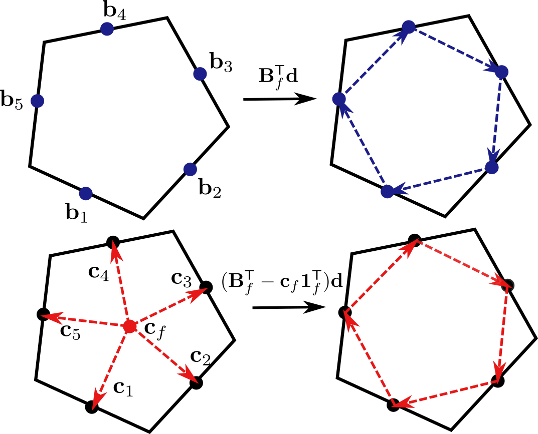
The previously presented Laplacians are closely related in their definitions of the inner product matrix for 1-forms. We will therefore shortly highlight some of the similarities and differences of the respective matrices. We already established that Alexa and Wardetzky’s matrix \(\tilde{\mv{M}}_f\) follows Brezzi et al.’s construction. \(\tilde{\mv{M}}_f\) is dependent on the choice of origin if regarded individually, however, combined with the difference matrix \(\mv{d}_f\) and its adjoint \(\mv{d}_f\tp\), this dependency vanishes. De Goes et al.’s equivalent eliminates this dependency immediately by regarding the midpoints relative to the respective centroid of the face as \(\mv{C}_f \in \R^{n_f \times 3}\), with row entries \(\mv{c}_i = \mv{b}_i - \mv{c}_f\). However, given a planar face, combining the matrices \(\mv{B}_f\tp\) and \(\mv{C}_f\tp\) with \(\mv{d}_f\) actually yields the same result, as visualized in Figure 5. Without the respective stabilization terms, both methods would lead to identical inner products since the remaining part of de Goes et al.’s method, namely \[\begin{align} -[\mv{n}_f]^2=\left(\mv{I}-\mv{n}_f\mv{n}_f\tp\right), \end{align}\] has no effect in this situation. Therefore, at least for planar polygons, the biggest difference between the inner product matrices are the stabilization terms.
Key Outcomes
For the computer graphics community, the main achievement of the two presented polygon Laplacians is to extend the MFD-based inner product stabilization from Brezzi et al. [11] to possible non-planar two manifolds embedded in 3D. While the individual mathematical derivations of the operators differ, they both introduce additional weighted stabilization terms in order to guarantee the crucial requirement of strict positive definiteness of the inner product matrices.
Demo: DEC-based Polygon Laplacians
Try computing mean curvature or geodesic distances using the two DEC-based polygon Laplacians (named “Alexa & Wardetzky Laplace” and “de Goes Laplace” in the demo). Observe how the choice of the hyper-parameter lambda influences the result.
Finite Elements Discretizations
The finite element method (FEM) is often used to approximate the solution \(u\) to a given PDE on a simplicial mesh with the help of a finite set of basis functions. The exact number depends on both the shape of the element and the order of the basis itself. In the linear case, we typically associate an individual shape function \(\varphi_i\) with the vertex \(\mv{x}_i\), also commonly referred to as node. Now, instead of solving the PDE directly, the objective changes to finding suitable coefficients \(u_i, \; i= 1,\dots,\abs{\mathcal{V}}\), that approximate the unknown solution \(u\) of the PDE with \[\begin{equation} \label{eq:FEM_interpolation} u(\mv{x}) = \sum_{i=1}^{\abs{\mathcal{V}}} u_i\varphi_i(\mv{x}). \end{equation}\] For example, a common problem solved with the finite element method is the Poisson equation \(-\Delta u = f\) for a known function \(f\). Given a surface mesh, the discretized PDE leads to a linear system \(\mv{L}\mv{u} = \mv{f}\) with a Laplace matrix \(\mv{L}\) that is defined as the integrated dot product of the gradients of the basis functions: \[\begin{align} \mv{L}_{ij} = \int_{\mathcal{M}} \langle\grad\varphi_i,\grad\varphi_j\rangle. \end{align}\] While a variety of different bases can be used to solve this system, for triangle meshes we focus on linear nodal shape functions that are defined piecewise per face and satisfy the Lagrange interpolation property already mentioned in Equation \(\eqref{eq:interpolation_property}\): \[\begin{align} \varphi_i(\mv{x}_j) = \begin{cases} 1 & \text{if } i=j, \\ 0 & \text{otherwise.} \end{cases} \end{align}\] Furthermore, we want them to satisfy additional properties within each element of the mesh in order to guarantee convergence under refinement [41]:
They have to be \(C^1\) continuous within the element and \(C^0\) across its boundaries.
For the basis to satisfy constant precision, the \(\varphi_i\) have to form a partition of unity \[\begin{equation} \label{eq:const_precision} \sum_{i=1}^{n_f} \varphi_i(\mv{x}) = 1. \end{equation}\]
They have to fulfill the linear reproduction property \[\begin{equation} \label{eq:lin_precision} \sum_{i=1}^{n_f} \varphi_i(\mv{x})\mv{x}_i =\mv{x} \end{equation}\] on planar polygons.
A standard set of basis functions meeting all these requirements are the piecewise linear hat functions on triangle meshes, also known as barycentric coordinates.
Demo: Barycentric Coordinates
The point \(\vec{x}\) in the center of the polygon can be represented by barycentric coordinates with respect to the polygon vertices \(\vec{x}_i\). The barycentric coordinates \(\varphi_i(\vec{x})\) with respect to polygon vertices \(\vec{x}_i\) (which are the FEM basis functions \(\varphi_i\) associated to the nodes \(\vec{x}_i\)) are displayed in the top right.
For general polygons, there exist a variety of generalized barycentric coordinates (GBC) [6, 30, 40, 43, 44], which are based on the idea to express any point within the polygon as weighted sum over its boundary nodes. This defines local shape functions that can be used in the finite element analysis. Extensive surveys [18, 29] have already discussed the benefits and properties of these shape functions.
Demo: Generalized Barycentric Coordinates
The point \(\vec{x}\) in the center of the polygon can be represented by barycentric coordinates with respect to the polygon vertices \(\vec{x}_i\). The barycentric coordinates \(\varphi_i(\vec{x})\) with respect to polygon vertices \(\vec{x}_i\) (which are the FEM basis functions \(\varphi_i\) associated to the nodes \(\vec{x}_i\)) are displayed in the top right.
Harmonic Coordinates
Since this report is more focused on the explicit construction of a Laplacian operator, we will not discuss shape functions based on GBC in the same depth, but rather explain one representative case, named the harmonic coordinates. While other methods like the maximum entropy coordinates [40] are very present in the FEM analysis on polytopes, we still chose the harmonic shape functions due to their numerous natural mathematical properties that makes them so well suited for FEM. This includes smoothness, non-negativity, the mean-value property and minimization of the Dirichlet energy [18, 52]. They can also be analyzed on arbitrary convex and non-convex polygons [77]. The only real drawbacks of these shape functions are them not having a closed form, and therefore requiring costly numerical integration, and that they are only defined on planar elements. In this section, we will review the construction of polygonal finite element shape functions based on the work of Joshi et al. [43] and Martin et al. [52]. As with the other methods, the properties of the harmonic coordinates will be further described in Section 7.
Harmonic Shape Functions on Planar Polygon Meshes
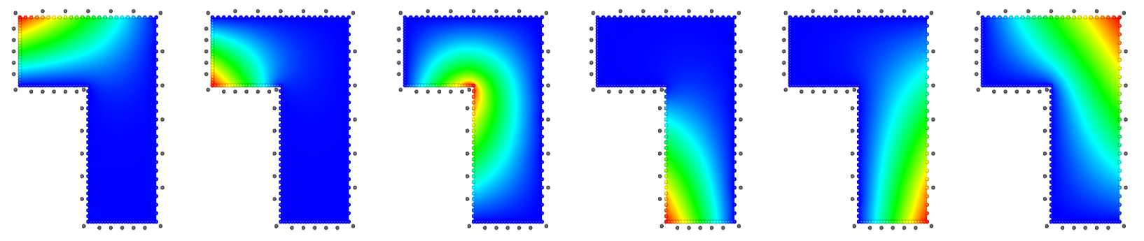
Given a mesh \(\mathcal{M}\) consisting of arbitrary polygons \(\F\), shape functions \(\varphi_i^f:f \rightarrow \R\), defined on a polygon \(f\in\F\), are called harmonic if they satisfy \(\Delta \varphi_i^f = 0\). In this case, they can be uniquely determined by specifying their function values \(b_i\) along the edges of the polygon as Dirichlet boundary conditions: \[\begin{equation} \label{eq:Laplace_equation} \begin{split} \Delta \varphi_i^f(\mv{x}) = 0 \quad &\text{for } \mv{x}\in f,\\ \varphi_i^f(\mv{x}) = b_i(\mv{x}) \quad &\text{for } \mv{x}\in \partial f. \end{split} \end{equation}\] In the linear case, the required Lagrange interpolation property and \(C^0\) continuity can be guaranteed by linearly interpolating the nodal values of \(\varphi_i^f\) along the boundary of the face. However, for polygons it is not possible to find a closed form for these shape functions and they have to be approximated numerically. This is why Martin et al. propose a scheme based on the method of fundamental solutions (MFS) [28] to determine the harmonic shape functions, although other methods are equally applicable. The core principle of MFS is to use an analytic fundamental solution \(\psi\) of the respective PDE, in our case the Laplace equation \(\eqref{eq:Laplace_equation}\), and approximate the sought solution through a linear combination of \(\psi\) centered at different source points \(\{\mv{k}_1,\dots,\mv{k}_n\}\) of the ambient Euclidean space. In our case, the fundamental solution to the 2D Laplace equation would be the radial basis function \[\begin{align} \psi(\norm{\mv{x}}) = \log(\norm{\mv{x}}), \end{align}\] which is well defined in \(\R^2\) except for one singularity at the origin. Translating this function to the previously chosen source points, we can approximate shape functions \({\phi}_i^f\) with \[\begin{equation} \label{eq:vanilla_mfs} \phi_i^f(\mv{x}) = \sum_{j=1}^n w_{ij} \psi\left(\norm{\mv{x}-\mv{k}_j}\right), \end{equation}\] which are then harmonic by construction.
The \(\psi_j(\mv{x}):= \psi(\norm{\mv{x}-\mv{k}_j})\) are also often referred to as kernels and their centers \(\mv{k}_j\) have to be placed outside of the face’s domain (see Figure 6) due to the singularity at \(\mv x = \mv k_j\). Martin et al. suggest a number of 3–5 kernels per edge distributed by a uniform sampling. However, in the current state, shape functions \({\phi}_i^f\) approximated via Equation \(\eqref{eq:vanilla_mfs}\) would not be able to exactly reproduce linear functions, violating the linear precision property. Therefore, Martin et al. add a linear polynomial \[\begin{equation} \label{eq:harmonic_shapefunctions} \varphi_i^f(\mv{x}) = \sum_{j=1}^n w_{ij} \psi(||\mv{x}-\mv{k}_j||) + \mv{s}_i\tp \mv{x} + r_i \end{equation}\] to guarantee that the function space spanned by the shape functions contains all linear functions. Linear polynomials are always harmonic, so \(\varphi_i^f\) still satisfies Equation \(\eqref{eq:Laplace_equation}\). In order to approximate the Dirichlet boundary constraints, we select \(m=3n\) uniformly sampled collocation points \(\mv{c}_i\) along the edges \(e_{kl}\) of the polygon to minimize the discretized boundary integral over the \(L_2\) error \[\begin{align} \int_{\partial f} \left(\varphi_i^f(\mv{x})-b_i(\mv{x})\right)^2 \approx \frac{1}{m} \sum_{j=1}^m \left(\varphi_i^f(\mv{c}_j)-b_i(\mv{c}_j)\right)^2. \end{align}\] This can be solved with the help of the following linear system \[\begin{equation} \ \label{eq:linsystem_harmonic} \begin{pmatrix} \psi_{11} & \cdots & \psi_{1n} & \mv{c}_1\tp & 1\\ \vdots & & \vdots & \vdots & \vdots\\ \psi_{m1} & \dots & \psi_{mm} & \mv{c}_m\tp & 1 \\ \end{pmatrix} \begin{pmatrix} w_{i1} \\ \vdots \\ w_{in}\\ \mv{s}_i\\ r_i \end{pmatrix} = \begin{pmatrix} b_i(\mv{c}_1) \\ \vdots \\ b_i(\mv{c}_m) \end{pmatrix}, \end{equation}\] where \(\psi_{ij} = \psi(||\mv{c}_i - \mv{k}_j||)\) and \(b_i(\mv{c}_j)\) contains the function value of the respective basis function at this point. Since the system is overdetermined , it has to be solved for the least-squares solution. Martin et al. recommend to use a QR factorization or the SVD pseudo inverse [34].
Stiffness and Mass matrix
Equipped with the shape functions described in the previous section, we are now able to express sought solutions of a PDE with the FEM interpolation scheme as described in Equation \(\eqref{eq:FEM_interpolation}\). The discretizations of both stiffness and mass matrix needed for the Laplacian can be obtained through \[\begin{equation} \label{eq:stiffness_harmonic} (\mv{L}_f)_{ij} = \int_f \langle \grad \varphi_i^f , \grad \varphi_j^f\rangle \d{\mv{x}}. \end{equation}\] and \[\begin{align} (\mv{M}_f)_{ij} = \int_f \varphi_i^f \cdot \varphi_j^f \d{\mv{x}}. \end{align}\] Note that this process requires numerical integration, since the gradients of the harmonic shape functions are not constant.
Demo: Harmonic Coordinates
Try computing a harmonic parameterization on this (rather simple) polygon mesh. Compare the performance of harmonic coordinates to the other polygon Laplacians. The required numerical integration of the harmonic shape functions makes it much more expensive.
Linear Virtual Refinement Method
Given the problems one has to deal with while working on general polygons, a rather pragmatic solution would be to simply refine the mesh into triangles. However, this can potentially break intended symmetry structures of the original tessellation and increase the dimension of linear systems if new vertices have to be added. The method presented by Bunge et al. [15] took inspiration from the simplicity of the triangle refinement, but proposed an in-between approach that avoids the downsides of an explicit refinement of the mesh.


Given a polygon mesh \(\mathcal{M}\), they introduce virtual vertices \(v_f\) into each (not necessarily planar) polygon \(f\). These are expressed as affine combinations of the original faces’ vertex positions \[\begin{equation} \vec{x}_{f} = \sum_{v_i \in f} w_i \;\vec{x}_i, \quad \text{ with } \sum_{v_i \in f} w_i =1. \end{equation}\] The additional vertices allow Bunge et al. to construct a virtual triangle mesh \(\mathcal{M}_{\vartriangle}\) by dividing each face into a triangle fan as shown in Figure 7. On this mesh, standard approaches like the cotan Laplacian (see Section 3) can be easily computed. However, in order to define operators working on the original mesh, Bunge et al. redistribute the values at the virtual vertices back to their associated polygon nodes. This is achieved by combining the affine weights \(\mv{w}_f=(w_1,\dots,w_{n_f})\) of each face into a local \((n_f+1) \times n_f\) prolongation matrix \[\begin{align} \label{eq:face_prolongation} \mv{P}_{ij}^f = \begin{cases} w_j & \text{for } i = n_f+1 \\ \delta_{ij} &\text{otherwise,} \end{cases} \end{align}\] which can be assembled into a global matrix \(\mv{P}\in \R^{(\abs{\mathcal{V}}+\abs{\F}) \times \abs{\mathcal{V}}}\) \[\begin{equation} \label{eq:global_face_prolongation} \mv{P}_{ij} = \begin{cases} 1 & \text{if } i = j \text{ and } i \leq \abs{\mathcal{V}} \\ w_{kj} & \text{if } i = \abs{\mathcal{V}}+k \text{ and } v_j \in f_k \\ 0 &\text{otherwise}, \end{cases} \end{equation}\] acting on the whole mesh. Using this matrix leads to a very easy refinement and coarsening process that allows Bunge et al. to define a polygon Laplacian, gradient and divergence operator on the original mesh: Given the global prolongation matrix \(\mv{P}\), they construct the cotangent mass and stiffness matrices \(\mv{M}_{\vartriangle}\) and \(\mv{L}_{\vartriangle}\) on the virtual triangle mesh \(\mathcal{M}_{\vartriangle}\) (see Equations \(\eqref{eq:triangle_mass_matrix}\) and \(\eqref{eq:triangle_stiffness_matrix}\)) and define the matrices for the original polygon mesh as \[\begin{equation} \label{eq:stiffness_prolongation} \mv{L} = \mv{P}\tp \mv{L}_{\vartriangle} \mv{P} \end{equation}\] and \[\begin{equation} \label{eq:mass_prolongation} \mv{M} = \mv{P}\tp \mv{M}_{\vartriangle} \mv{P}. \end{equation}\] As for the Laplacian, they compute the gradient and divergence operators \(\mv{G}_{\vartriangle}\) and \(\mv{D}_{\vartriangle}\) on \(\mathcal{M}_{\vartriangle}\) by using the simplicial definitions in Equations \(\eqref{eq:triangle_gradient}\) and \(\eqref{eq:triangle_divergence}\) express the polygon operators as \[\begin{align} \mv{G} = \mv{G}_{\vartriangle} \mv{P} \end{align}\] and \[\begin{align} \mv{D} = \mv{P}\tp \mv{D}_{\vartriangle} = \mv{P}\tp \mv{G}_{\vartriangle}^{\mathsf{T}}\hat{\mv{M}}_{\vartriangle}. \end{align}\] Combining both polygon gradient and divergence leads once again to the stiffness matrix \(\mv{L}\) and is therefore consistent with the previous discretization. The remaining question addressed by Bunge et al. [15] is the placement of the virtual vertex. Given that positions outside of the (planar) polygon’s boundary would lead to flipped virtual triangles with bad numerical properties, they suggest the virtual vertex to be the unique minimizer of the sum of squared triangle areas of the refined face. This is motivated by the fact that for a planar star-shaped polygon the point almost always lies within the kernel of the polygon, leading to virtual triangles with positive areas. Finding the vertex position can be directly expressed as minimization problem over the weight vector \(\vec{w}_f = (w_1,\dots,w_{n_f})\tp \in \R^{n_f}\) with \[\begin{align} \label{eq:area_minimizer} \vec{w}_f =& \arg \min_{\vec{w}} \sum_{i=1}^{n_f} \text{area}\left(\vec{x}_i,\vec{x}_{i+1}, \sum_{j =1}^{n_f} w_j \;\vec{x}_j\right)^2 \\ & \text{such that } \sum_{j =1}^{n_f} w_j =1. \end{align}\] However, for faces with valence higher than three, this system is under-constrained and several sets of weights are able to represent the point. The authors therefore add the constraint that the weight vector should have minimal \(L_2\) norm, which leads to a unique solution that encourages a more uniform distribution among the weights and can be solved with a linear system.
While these weights are simple to compute, they do not necessarily yield a well-shaped virtual triangle fan. To this end, Bunge et al. [14] propose an alternative vertex position and corresponding weights that minimize the harmonic index [8, 56], as a lower harmonic index can be linked to better-shaped triangles and more favorable stiffness matrix conditioning. However, it requires an iterative optimization strategy for the virtual vertex, which is less performant and more complex to implement.
Furthermore, both approaches still suffer from the regular cotangent Laplacian discretization, as (near-)degenerate polygons do not allow well-shaped triangle fans, independent of the virtual vertex. This can be alleviated by also applying the D-TFEM scheme (see Section 3.3.2), as demonstrated by Wagner and Botsch [73]. They show that even completely degenerate triangles in the virtual triangle fan can still yield decent results.
Finite Element Shape Functions
Drawing the connection to traditional FEM methods, the previously defined prolongation weights allow Bunge et al. [15] to define a set of local shape functions \(\{\varphi_1^f,\dots,\varphi_{n_f}^f\}\) associated with the vertices of the polygon \(f\): If \(\varphi_i^{\vartriangle}\) are the \((n_f+1)\) Lagrange basis functions (see Section 3) defined on the refined polygon, one can construct coarse shape functions \(\varphi_i^f\) associated with the polygon nodes as \[\begin{equation} \label{eq:coarsened_shapefunction} \varphi_i^f = \varphi_i^{\vartriangle} + w_i\varphi_f^{\vartriangle}, \quad i=1,\dots,n_f. \end{equation}\] Here, \(\varphi_f^{\vartriangle}\) refers to the Lagrange basis function associated with the virtual vertex \(v_f\) and \(w_i\) is the respective entry in the affine weight vector \(\mv{w}_f\) previously used for the prolongation matrix. Integrating these shape functions over the polygon mesh as described in Section 5.1.2 would lead to the same discretized stiffness and mass matrices as defined in Equations \(\eqref{eq:stiffness_prolongation}\) and \(\eqref{eq:mass_prolongation}\). Given their construction, Bunge et al.’s shape functions are linear within each virtual triangle and can be integrated analytically, in contrast to the harmonic shape functions, which require more expensive numerical integration.
Similarities to DEC
Interestingly, combining the prolongation matrix \(\mv{P}\) with the standard Lagrange basis functions \(\{\varphi_1^{\vartriangle},\dots \varphi_{\abs{\V_{\vartriangle}}}^{\vartriangle}\}\) defined on the refined triangle mesh allows us to reinterpret the construction of the stiffness matrix \(\mv{L}\) in Equation \(\eqref{eq:stiffness_prolongation}\) as \[\begin{align} \mv{L} = \mv{d}_{\E}\tp \star^1 \mv{d}_{\E}, \end{align}\] which follows the same structure as the operators presented in Section 4. Here \(\star^1\) denotes a polygon equivalent of the so-called Hodge star operator acting on 1-forms, and the matrix \(\mv{d}_{\E} \in \R^{\abs{\E}\times \abs{\mathcal{V}}}\) is the discrete differential operator \[\begin{align} (\mv{d}_{\E})_{kl} = \begin{cases} -1 & l=i \\ 1 & l=j\\ 0 & \text{ otherwise} \end{cases} \end{align}\] taking 0-forms to 1-forms acting on edges (in contrast to the previously used coboundary operator \(\mv{d}\) that projects to halfedges). As in Equation \(\eqref{eq:coboundaryoperator}\), the indexing addresses the \(k\)-th row of the operator, this time associated with the \(k\)-th edge \(e_{ij}\in \E\). Bunge et al. [15] define a suitable polygon Hodge star by first constructing the respective basis functions for 1-forms: Since the coarse polygon basis functions \(\{\varphi_1,\dots \varphi_{\abs{\mathcal{V}}}\}\) are associated with the vertices of the mesh \(\mathcal{M}\), they form a set of 0-forms and can be expressed as \[\begin{align} \varphi_j = \sum_{i=1}^{\abs{\V_{\vartriangle}}}\mv{P}_{ij}\varphi_i^{\vartriangle}. \end{align}\] By construction, these bases form a partition of unity. Therefore, they can be used to define a set of polygon Whitney bases [3, 76] for 1-forms, with \[\begin{align} \varphi_{ij} = \varphi_i \cdot \mv{d}_{\E}\varphi_j- \varphi_j \cdot \mv{d}_{\E}\varphi_i = \sum_{l=1}^{\abs{\V_{\vartriangle}}}\sum_{k=1}^l\mv{P}_{ki}\mv{P}_{lj}\varphi_{kl}^{\vartriangle}, \end{align}\] being a 1-form associated to the polygon edge \(e_{ij}\in \mathcal{E}\). In order to define a prolongation operator that maps 1-forms from polygon edges to edges on the refined triangle mesh, Bunge et al. define a second prolongation matrix \(\mv{P}^1 \in \R^{\abs{{\E}_{\vartriangle}} \times \abs{\mathcal{E}}}\) as \[\begin{align} \mv{P}^1_{(ij)(kl)} = \mv{P}_{ik}\mv{P}_{jl}, \end{align}\] with \((ij)\) indicating the row associated to the edge \(e_{ij}^{\vartriangle} \in \E_{\vartriangle}\) on the refined mesh and \((kl)\) the index of the respective coarse polygon edge \(e_{kl} \in \E\). This matrix can be combined with the discrete Hodge star \(\star^1_{\vartriangle}\) on the refined triangle mesh, giving us \[\begin{align} \mv{M}_1 = \star^1 = \left(\mv{P}^1\right)\tp\star^1_{\vartriangle}\mv{P}^1 \end{align}\] and \[\begin{align} \mv{L} = \mv{d}_{\E}\tp \left(\mv{P}^1\right)\tp\star^1_{\vartriangle}\mv{P}^1 \mv{d}_{\E}. \end{align}\] The question is if this inner product matrix \(\mv{M}_1\) satisfies the same desiderata as for example the matrices presented by Alexa and Wardetzky [1] and de Goes et al. [32], which remains to be investigated.
Key Outcomes
The presented FEM methods can, just like the previously discussed Mimetic Polygon Laplacians, be applied to any type of polygon surface mesh. However, the harmonic shape functions are restricted to planar polygons, while the linear virtual refinement method is able to deal with non-planar elements. Furthermore, besides being able to construct all the operators we already described, having explicit shape functions allows us to interpolate any given function within the polygons if we know its values at the vertex positions. In relation to the MFD operators, since the virtual refinement method allows for a reinterpretation of the Laplacian in the same inner product structure, future analysis could further investigate the relation between FEM and MFD approaches and their different qualities.
Demo: Virtual Refinement
Play around with the Laplacian from virtual refinement (named “PolySimple” in the demo, due to the original paper title “Polygon Laplacian made Simple”). Observe that it doesn’t require tuning a hyper-parameter and that it is rather efficient.
Finite Volume Discretizations
The finite volume method (FV) was originally introduced by Dusinberre [25, 26] for the heat equation and can be used on all differential equations that can be expressed through the divergence operator. It follows the idea that the integral of a differential over a small volume can be expressed as a surface integral of the fluxes over the boundary of the same cell [61]. As the MFD, finite volume discretizations can be considered mimetic since they try to enforce balance equations for mass, momentum, and energy on each cell [49], conservation properties that make them well suited for fluid mechanic problems. However, the basic derivation of the 2D Laplace operator with FV assumes a Delaunay triangle mesh, more specifically orthogonal dual and primal edges, in order to prevent negative coefficients. To avoid this restriction, Bunge et al. [16] used a special polygonal variant of the FV, called Discrete Duality Finite Volume (DDFV) [20, 24, 37, 38] and combined this technique with their previously described virtual triangle refinement to define a gradient, divergence and Laplacian operator for polygonal meshes.
Discrete Duality Finite Volume Method
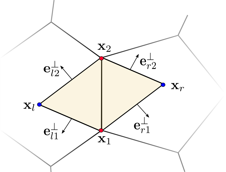
We will shortly revisit the definition of a 2D gradient operator constructed with the DDFV approach. Given a planar polygonal surface mesh \(\mathcal{M}\), we consider a second set of vertices, called dual vertices \(\mathcal{V}^*\), associated with the barycenter of each face \(f\in \mathcal{F}\). For each edge \(e \in \mathcal{E}\), they are able to span a so-called diamond cell \(D\), consisting of the vertex pair \(v_1,v_2\) connected by \(e\) and the dual vertices \(v_l, v_r\) associated to the faces adjacent to the edge (see Figure ). The diamond cell always forms a rectangular shape with edge vectors \(\mathbf{e}_{ij} = \mv{x}_j-\mv{x}_i\) in \(\R^2\) assigned to the edge tuples \((i,j)\in D\). On these diamonds, the DDFV method uses Stokes’ theorem in order to define a local gradient for a function \(u\) in the following way \[\begin{align} \iint_{D} \grad u(\mv{x}) \d{\mv{x}} &= \int_{\partial D} u(\mv{x})\, \mv{n}(\mv{x}) \d{\mv{x}}\\ &= \sum_{(i,j) \in \partial D} \frac{\mv{e}_{ij}^\perp}{\norm{\mv{e}_{ij}}} \, \int_0^1 \norm{\mv{e}_{ij}} \left((1-t)u_i+t u_j\right) \d{t}\\ &=\sum_{(i,j) \in \partial D} \mv{e}_{ij}^\perp \frac{u_i+u_j}{2}. \label{eq:grad-deriv} \end{align}\] Here \(u_i\) denotes the function values associated to the vertex \(v_i\) and \(\vec{n}(\mv{x}) \in \R^2\) is an outward pointing normal vector at point \(\mv{x}\) along the boundary of the diamond. Therefore, the gradient operator can be solely expressed through the four outward rotated edge vectors of the respective diamond. One of the many benefits of the DDFV method is the discrete duality property between its discrete gradient and divergence operators, also known as Green’s “integration-by-parts” formulas [2, 49]. This property is an essential part of the finite volume setting.
Diamond Laplace for Surface Meshes
Bunge et al. [16] adapt the previously defined DDFV gradient operator in two ways to extend it to polygon surface meshes embedded in 3D:
First, they reduce the systems’ dimension by expressing the values at the dual vertices as affine combinations of the original primal vertices with the help of the previously introduced face prolongation matrix \(\mv{P}\) (see Equation \(\eqref{eq:global_face_prolongation}\)). As in Section 5.2, the position of the dual vertices is the minimizer of the sum of squared triangle areas of the refined face.
Second, they define an intrinsic gradient operator associated with the (not necessarily planar) diamond cells, allowing them to directly apply the formula defined in Equation \(\eqref{eq:grad-deriv}\).
Given a diamond cell \(D\) with vertices \((v_1,v_2,v_l,v_r)\) embedded in \(\R^3\), the first objective is to isometrically unfold the planar triangles along their shared edge into a plane. The new 2D coordinates can then be used to construct the diamonds gradient operator \(\mathbf{G}_D \in \R^{2\times 4}\). For each column \(i\) associated with a vertex it is defined as \[\begin{align} \label{eq:surface_diamondgradient} \mathbf{G}_D(:,i) = \frac{1}{2 \abs{D}} \sum_{(i,j)\in \partial D} \tilde{\mv{e}}_{ij}^{\bot}, \end{align}\] where \(\abs{D}\) denotes the diamond’s area and \(\tilde{\mv{e}}_{ij}^{\bot} \in \R^2\) orthogonal vectors to the intrinsic 2D diamond edges. These local gradient matrices are then assembled into a global operator \(\mathbf{G}_{\diamond}\in \R^{2\abs{\mathcal{E}}\times (\abs{\mathcal{V}}+\abs{\mathcal{F}})}\) defined on the refined triangle mesh \(\mathcal{M}_{\vartriangle}\). Combined with the surface prolongation matrix \(\mathbf{P}\) (see Equation \(\eqref{eq:global_face_prolongation}\)), we obtain a gradient operator for the original polygon mesh through \[\begin{equation} \mathbf{G} = \mathbf{G}_{\diamond} \mathbf{P}. \end{equation}\] This operator maps function values \(u_i\) associated with the primal vertices \(v_i \in \mathcal{V}\) to intrinsic gradient vectors \(\grad u|_D \in \R^2\) associated to the diamond cells spanned on the virtual triangle mesh \(\mathcal{M}_{\vartriangle}\). Following the DDFV discretization of the divergence, Bunge et al. [16] define their diamond divercence operator as \[\begin{align} \mv{D} = \mv{P}\tp\mv{G}_{\diamond}\tp \hat{\mv{M}}_{\diamond} \end{align}\] where \(\hat{\mv{M}}_{\diamond} \in \R^{2\abs{\mathcal{E}}\times 2 \abs{\mathcal{E}}}\) is a diagonal matrix containing the diamond \(D_i\)’s area \(\abs{D_i}\) in its diagonal entries with indices \(2i\) and \(2i+1\). The final stiffness matrix is then directly derived from its definition as the divergence of the gradient and given by \[\begin{align} \mv{L} = \mv{D}\mv{G} = \mv{P}\tp\mv{G}_{\diamond}\tp \hat{\mv{M}}_{\diamond} \mathbf{G}_{\diamond} \mathbf{P}, \end{align}\] mapping from vertices to vertices. The diamond version of the mass matrix required for the strong formulation \(\mathbb{L}\) of the Laplacian is defined as \[\begin{align} \mv{M} = \mathbf{P} \tp \mathbf{M}_{\diamond} \mathbf{P}. \end{align}\] It is derived from the standard DDFV diagonal mass matrix \(\mathbf{M}_{\diamond} \in \R^{(\abs{\mathcal{V}}+\abs{\F})\times(\abs{\mathcal{V}}+\abs{\F})}\) that distributes the diamond areas to the primal and dual vertices: \[\begin{align} \label{eq:diamond_mass_surface} (\mv{M}_{\diamond})_{ii} = \begin{cases} \sum_{D \ni v_i} \frac{\abs{D}}{4}& \text{if } v_i \in \mathcal{V} \\ \sum_{D \ni v_i} \frac{\abs{D}}{4}& \text{if } v_i \in \mathcal{V}^* \\ 0 &\text{otherwise}. \end{cases} \end{align}\]
Key Outcomes
As for the FEM methods, the diamond Laplacian can be applied to surface meshes with possible non-planar faces. In contrast to the previous operators, the influence of the DDFV background causes its focus to lie more on the construction of a plausible gradient and divergence operator, which can both be constructed intrinsically. The diamond structure combined with the prolongation steps leads to a larger local neighborhood, which can yield more accurate results (see Section 8), but also causes denser and therefore more costly system matrices.
Properties of the Polygon Laplacians
In this section, we analyze each of the previously introduced polygon Laplacians based on the properties established by Wardetzky et al. [75] (see Section 2.1). Since all methods fail to satisfy the maximum principle, but are otherwise able to retain the remaining properties, we will structure the upcoming section accordingly. Therefore, this section will focus more on notable differences within the derivations and proofs of the individual properties instead of differences between the actual operators themselves.
Symmetry
Each of the presented Laplace operators fulfills symmetry by construction. As the products of individual symmetric or diagonal matrices, the respective inner product matrices \(\mv{M}_f\) introduced in both [1] and [32] are symmetric as well. Therefore, given that the local stiffness matrix is defined as \(\mv{d}_f\tp \mv{M}_f \mv{d}_f\), it and the globally assembled weak form fulfill this property.
Since the FEM stiffness matrix is defined as the integrated dot product of the shape functions’ gradients, the property follows naturally for the operators introduced by [52] and [15].
In case of the diamond Laplacian, it follows from the definition of the weak form as \[\begin{align} \mv{L} = \mv{D}\mv{G} = \mv{P}\tp\mv{G}_{\diamond}\tp \hat{\mv{M}}_{\diamond} \mathbf{G}_{\diamond} \mathbf{P} \end{align}\] and \(\hat{\mv{M}}_{\diamond}\) being a diagonal matrix.
Locality
All methods, with the exception of [16], define their involved matrices or shape functions locally per polygon. This implies that their respective influence is restricted to the boundary of the individual elements. Therefore, for operators discretized with linear degrees of freedom, the stencil of the Laplacian associated with a single vertex \(v_i\) involves all face vertices of the polygons where \(v_i\) itself is a part of, which leads to a local neighborhood. However, the diamond Laplacian has a larger stencil than the other operators. Since the diamond structure connects adjacent cells on the refined mesh and the prolongation process distributes values at virtual vertices back to all original face nodes, its neighborhood for a vertex \(v_i\) consists of the same vertices as the other methods, and additionally those that are part of a face sharing an edge with the primitives surrounding \(v_i\).
Linear Precision
In contrast to the previous two properties, linear precision does not automatically follow from each operator’s construction and must be proven individually.
Alexa and Wardetzky.
For the Laplacian introduced by Alexa and Wardetzky, similarly to the cotan Laplacian, the proof is based on the area gradient of the polygon with respect to its vertices. Consider the vertex \(v_i\) to lie in a planar neighborhood. Starting with Equation \(\eqref{eq:linear_precision}\), we have to focus on two terms in order to show linear precision for Alexa and Wardetzky’s operator: \[\begin{align} \tilde{\mv{L}}_f \mv{X}_f = \mv{d}_f\tp \tilde{\mv{M}}_f\mv{d}_f\mv{X}_f, \end{align}\] where \[\begin{align} \tilde{\mv{L}}_f := \mv{d}_f\tp \tilde{\mv{M}}_f\mv{d}_f \end{align}\]with \(\tilde{\mv{M}}_f\) being the inner product matrix defined by Brezzi et al. [11] (see Equation \(\eqref{eq:innerProduct_Brezzi}\)), and \[\begin{align} \mv{d}_f\tp \mv{C}_{\bar{f}} \mv{U}_{\bar{f}} \mv{C}_{\bar{f}}\tp\mv{d}_f\mv{X}_f. \end{align}\] As shown in Equation \(\eqref{eq:Alexa_linprecision}\), the latter term vanishes for planar polygons, leaving us with the remaining part \(\tilde{\mv{L}}_f \mv{X}_f\). As shown in Lemma 3 in the original paper, the \(i\)-th row of this matrix is equivalent to the polygon’s area gradient at vertex \(v_i\): \[\begin{align} \grad_{\mv{x}_i}\abs{f} = \left(\tilde{\mv{L}}_f \mv{X}_f\right)_i. \end{align}\] Therefore, the expression \((\mv{L}\mv{X})_{i}\) is equal to the sum over the area gradients of the adjacent faces with respect to the vertex \(v_i\). Given that the neighborhood is planar, this sum becomes zero since moving the vertex in any direction in the plane would leave the area unchanged.
De Goes et al.
For de Goes et al.’s Laplacian [32], we proceed in the same fashion as for Alexa and Wardetzky and consider the individual terms of the inner product matrix, starting with the projection: \[\begin{equation} \mv{P}_f \mv{d}_f \mv{X}_f = \mv{P}_f\mv{E}_f. \end{equation}\] As mentioned by the authors, \(\mv{P}_f\) actually eliminates all discrete 1-forms in the image of \[\begin{align} \mv{V}_f^{\flat}=\mv{E}_f \left(\mv{I}-\mv{n}_f\mv{n}_f\tp\right). \end{align}\]Therefore, the projection term vanishes if applied to \(\mv{E}_f\). As described in Section 4.4, since the vertex \(v_i\) is surrounded by planar polygons, the remaining inner product term is equal to \(\tilde{\mv{L}}_f \mv{X}_f\) for each individual face \(f\), allowing for the same area gradient interpretation.
Harmonic Coordinates.
In the finite element theory, a common practice is to ensure that shape functions pass the so-called patch test, which verifies if they are able to fulfill the linear precision property we defined in Equation \(\eqref{eq:lin_precision}\). A variant of the requirements the shape functions have to meet in order to pass the patch test are the exact same as our definition of the linear precision property for Laplacians [79]. Therefore, given that the harmonic shape functions are linearly precise, Martin et al.’s Laplacian satisfies this property as well. In fact, as discussed by the authors in the original paper, the linear polynomial introduced in Equation \(\eqref{eq:harmonic_shapefunctions}\) is crucial to guarantee exact linear precision, and therefore this property, independent of the number of chosen kernels.
Linear Virtual Refinement Method.
The linear precision property is satisfied if the following expression \[\begin{align} (\mv{L}\mv{u})_i = 0, \end{align}\] holds for all interior vertices \(v_i\) where the incident polygons \(f_j \ni v_i\) are co-planar and the values of \(\mv{u}\) in the one-ring of \(v_i\) are obtained by sampling a linear function on the plane. Given that the elements surrounding the interior vertex \(v_i\) are co-planar, the same must hold for the refined triangles of these primitives, since the position of the virtual vertex is an affine combination of the existing face vertices. The cotangent Laplacian has linear precision, so any linear function \(\mv{u}\) sampled at the vertices and prolonged to the refined mesh \(\mv{u}_{\vartriangle} = \mv{P} \mv{u}\) satisfies \[\begin{align} (\mv{L}_{\vartriangle}\mv{u}_{\vartriangle})_i = 0 \end{align}\] for the interior vertex \(v_i\) and all virtual vertices of its surrounding faces. These are exactly the values on the refined mesh that account for the value of the polygon Laplacian at \(v_i\), since each value associated to the virtual vertices is redistributed to the original nodes of the mesh by applying \(\mv{P}\tp\) to \(\mv{L}_{\vartriangle}\mv{u}_{\vartriangle}\). Them all being zero gives us \((\mv{L}\mv{u})_i =0\).
However, when also applying D-TFEM [73], the triangular Laplacian does not necessarily fulfill this property, as discussed in Section 3.3.2. Consequently, the polygon Laplacian also fails to satisfy the property.
Diamond Laplacian.
Knowing that the DDFV Laplacian \(\mv{G}_{\diamond}\tp \hat{\mv{M}}_{\diamond} \mv{G}_{\diamond}\) satisfies linear precision on the refined mesh [19, 24, 37], applying the full-rank prolongation matrices preserves this property.
Positive Semi-Definiteness and Null Space
For Martin et al.’s and Bunge et al.’s operators [15, 52], given that their Laplacians follow the standard FEM approach, the respective stiffness matrices fulfill both properties by construction and do not require individual proofs.
In case of Alexa and Wardetzky [1] and de Goes et al. [32], the strict positive definiteness of their respective inner product matrices \(\mv{M}_1\) is a fundamental building block in their derivation process, which leads to a kernel that contains only the zero vector. Furthermore, given its construction, the kernel of the coboundary operator \(\mv{d}\) contains only constant functions. Combining these two matrices into \(\mv{d}\tp \mv{M}_1 \mv{d}\) therefore yields a positive semi-definite stiffness matrix with a one-dimensional kernel consisting of constant functions.
For the diamond Laplacian, the diagonal matrix \(\hat{\mv{M}}_{\diamond}\) is symmetric positive definite. The prolongation matrix \(\mv{P}\) has full rank and therefore the constructed stiffness matrix is also positive semi-definite. However, the dimension of the null space requires further explanation. While it is obvious that constant functions, given its definition, lie in the kernel of the gradient, it remains to be shown that they are the only ones that do. As mentioned by Bunge et al. [16], both the gradient of a minimal diamond and a 2D diamond cell can be interpreted as the gradient of an affine function fitted to the function values of the edge midpoints of the respective cell. The gradient will therefore vanish if all function values associated to the midpoints are identical. However, this can only be satisfied if the function values at the dual and primal vertices of the respective diamond are identical as well. Furthermore, since the diamonds share the function values with their adjacent cells along the common boundary element, this requirement propagates through the complete mesh, leaving only room for constant functions.
Maximum Principle
As previously mentioned, all of the presented Laplacians are not able to fulfill the maximum principle for general meshes. In case of the Diamond Laplacian, failing to satisfy the maximum principle is a known limitation of the DDFV scheme [59], which can not be rectified by applying the prolongation matrices. All other methods reproduce the cotan Laplacian on triangle meshes, which is also not able to retain this property as discussed in Section 3.
Evaluation
In this section, we compare the performance of the presented Laplace operators in a number of different computer graphics applications for surface meshes. We are interested in the influence of the respective parameters \(\lambda\) described by Alexa and Wardetzky [1] and de Goes et al. [32] and how they affect the quality of the inner product matrix. Therefore, we analyze a selection of values besides the recommended choices of the authors. Concerning the placement of the virtual vertices, we follow the recommendations of Bunge et al. [15, 16] and use the squared triangle area minimizer, respectively. For the harmonic shape functions [52], we noticed that the number of chosen kernels and control points strongly affects the results on our chosen test meshes (see Figure 9). We analyzed different numbers of kernels with \(m=4n\) collocation points instead of the recommended ratio of \(m=3n\) from the original paper, since it yielded slightly more accurate results in our setting. Based on this evaluation, we increased the number of edge kernel/collocation points for surface meshes to 20/90. The choice was also influenced by the numerical costs involved in using more samples. The triangles used for the numerical integration are the same as the virtual elements used for the virtual refinement method. Given that the integration of the shape functions is not exact, using a more elaborate tessellation technique could further improve the results.
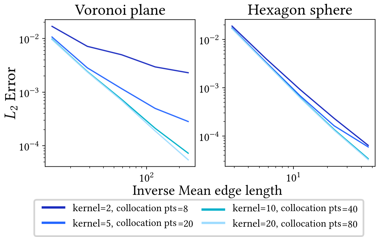
Poisson Equation
We analyze the convergence behavior of the different Laplacians by solving the Poisson equation \(-\Delta u = f\) with Dirichlet boundary conditions on various refined tessellations of the unit square. We chose the 2D Franke test function [31] for the right hand side \(f\) and solve the discrete system \[\begin{align} \mv{L} \mv{u} = \mv{M}\mv{b}, \end{align}\] with \(\mv{b} \in \R^{\abs{\mathcal{V}}}\) containing the values of the analytic Laplacian \(\Delta f\) of the test function sampled at the vertices. The solution \(\mv{u}\) is then compared to the analytic values of \(f\). The exact formula of the Franke test function is \[ \begin{split} f_{\mathrm{2D}}\of{x,y} \;=\; &\frac{3}{4} \mathrm{e}^{-\frac{(9x-2)^2+(9y-2)^2}{4}} +\frac{3}{4} \mathrm{e}^{-\frac{(9x+1)^2}{49}-\frac{9y+1}{10}} \\ +&\frac{1}{2} \mathrm{e}^{-\frac{(9x-7)^2+(9y-3)^2}{4}} -\frac{1}{5} \mathrm{e}^{-(9x-4)^2-(9y-7)^2}. \end{split} \]
Figure 10 showcases the \(L_2\) error rates from solving the Franke Poisson system on different surface meshes. Each Laplacian is able to reproduce the expected quadratic convergence rate across all tessellations. In terms of accuracy, both operators introduced by Alexa and Wardetzky [1] and de Goes et al. [32] are able to produce high quality results for \(\lambda = 1\) on quad and Voronoi meshes. On concave surfaces, de Goes et al. with parameter \(\lambda = 0.5\) yields the lowest errors, closely followed by the operator presented by Bunge et al. [15]. The Diamond Laplacian consistently maintains low error rates and since it is not reduced to the cotangent Laplacian, it also yields better results on the triangle grid.
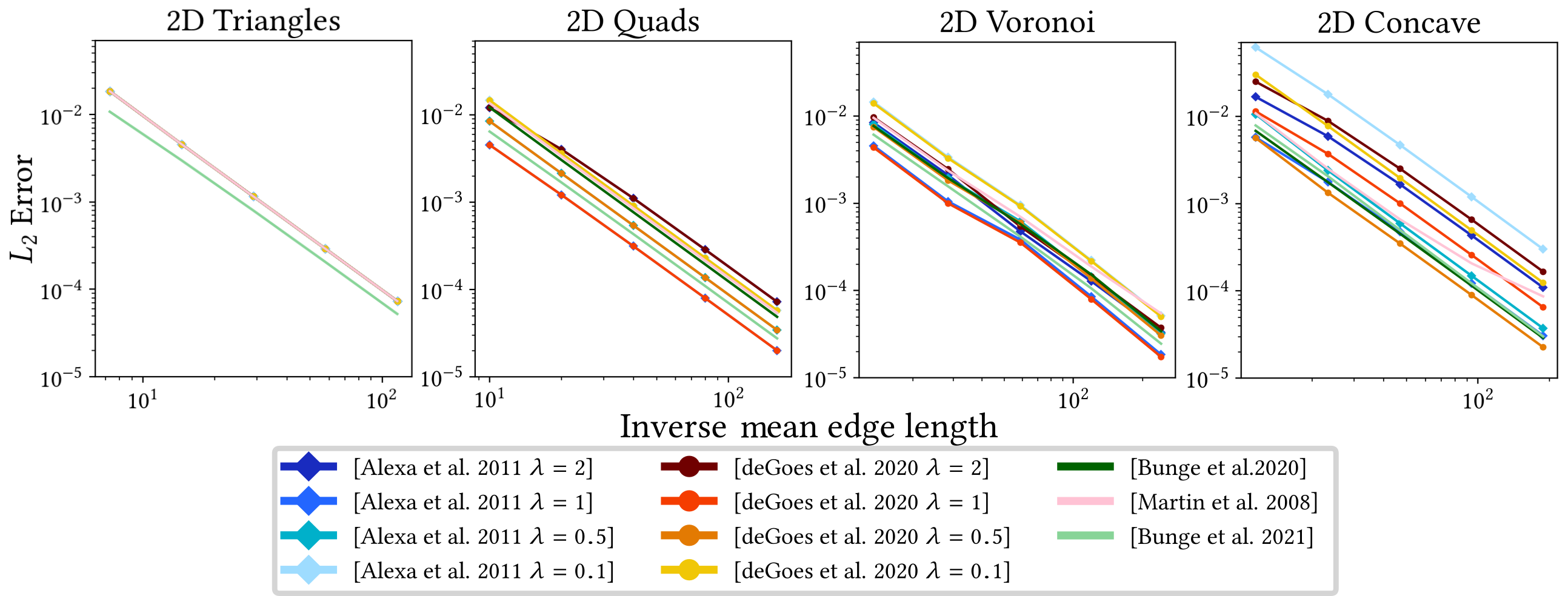
Spherical Harmonics
The eigenfunctions of the Laplacian on the unit sphere \(\mathcal{S}^2\) are called the spherical harmonics \(Y^m_l : \mathcal{S}^2 \rightarrow \R\) with eigenvalues \(-l(l+1)\). Using the fact that \(Y^m_l\) are eigenfunctions, we can solve for \(\mv{u} \in \R^{\abs{\mathcal{V}}}\): \[\begin{align} & \mv{u} = \mv{M}^{-1}\mv{L} \mv{y}_l^m \\ \Leftrightarrow \quad &\mv{M} \mv{u} = \mv{L}\mv{y}_l^m \end{align}\] and rescale the solution with the respective eigenvalue. The entries of \(\mv{y}_l^m\in \R^{\abs{\mathcal{V}}}\) denote the function values of \(Y^m_l\) sampled at the vertices. We can measure the error of \(\mv{u}\) being an eigenfunction to the presented Laplace operators by evaluating \[\begin{align} \norm{\mv{y}_l^m + \frac{1}{l(l+1)} \mv{u}}^2_{\mv{M}} \end{align}\] for a selected frequency with non-zero eigenvalue. The \(L^2\) norm is computed with respect to the inner product induced by the mass matrix \(\mv{M}\).
Figure 11 displays the deviation of the solution from the analytic function values of \[\begin{align} Y^3_2(x,y,z) = \frac{1}{4}\sqrt{\frac{105}{\pi}}(x^2-y^2)z \end{align}\] with eigenvalue \(-12\). The linear virtual refinement method yields some of the lowest error rates especially for hexagons, while the harmonic shape functions yield very good results on the concave tessellation, which are only surpassed by the Diamond Laplacian. As for the operators presented by Alexa and Wardetzky and de Goes et al., choosing lower \(\lambda\) for the stabilization term leads to the most accurate results, with \(\lambda =0.5\) being one of the most consistent options. The effect of chosen sample points on the harmonic shape functions and their possible numerical artifacts can be observed in Figure 9. We analyzed different kernel/collocation point samples for both the Franke as well as the spherical harmonics Poisson solve and observed the expected behavior of lower kernel numbers influencing both error and convergence rate.
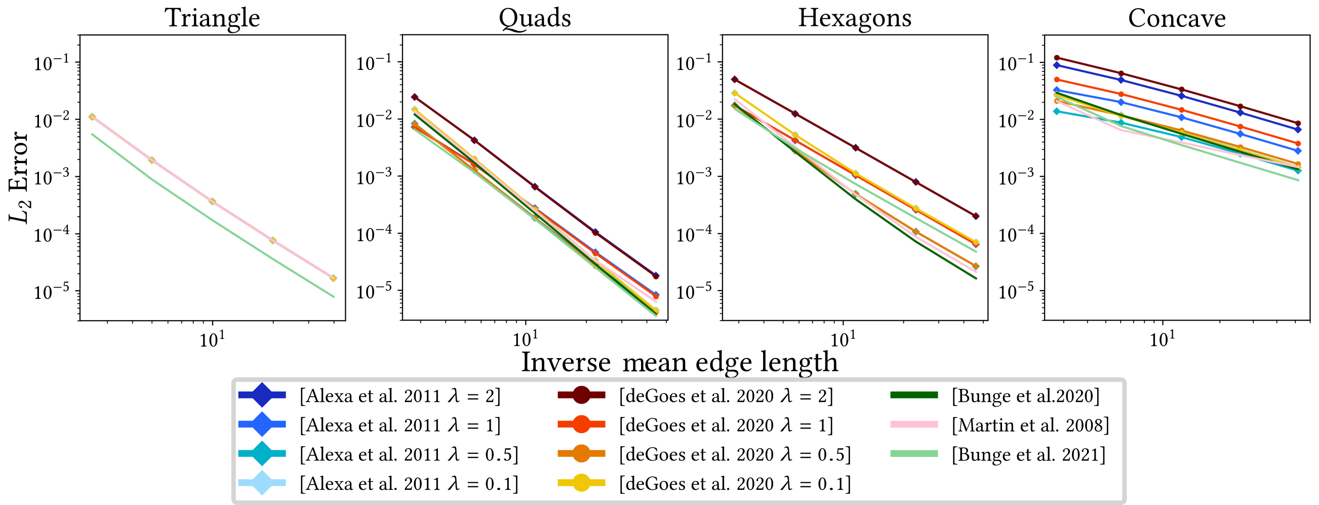
Eigenvalues
Given that the spherical harmonics have an analytic expression for their eigenvalues, we can solve the generalized eigenvalue problem \[\begin{align} \label{eq:generalized_eigenvalues} \quad &\mv{L}\mv{u}=\tilde{\lambda}\mv{M}\mv{u} \end{align}\] for the eigenvalues \(\tilde{\lambda}\) of the discrete Laplacians and compare them to the analytic values. Figure 12 shows the first eigenvalues of each polygon Laplacian obtained on different spherical meshes. For both Alexa and Wardetzky’s and de Goes et al.’s operators, a value of \(\lambda = 1\) leads to very accurate results. Using smaller values for the parameter leads to larger eigenvalues, while higher \(\lambda\) yield results that are lower than the correct solution. The other methods lead to relatively similar deviations with eigenvalues that display the expected “stair-like” appearance, but are too large in the higher frequencies. The highest and lowest values for \(\lambda\) start to lose the stair-like pattern for the eigenvalues.
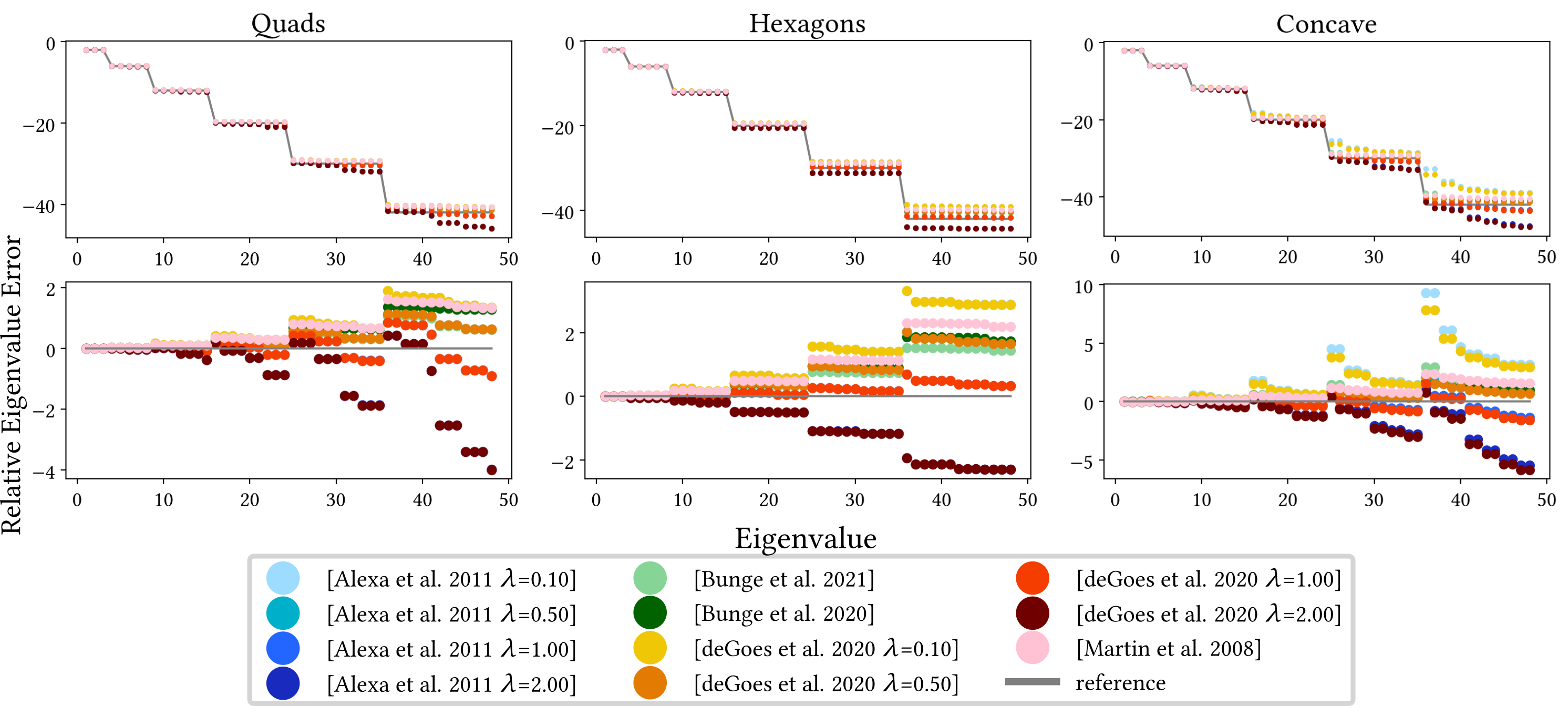
Geodesics in Heat
In order to assess the quality of the divergence and gradient operators, we evaluate them in the context of the geodesics in heat method presented by Crane et al. [21]. Given the \(i\)-th unit vector \(\mv{e}_i \in \R^{\abs{\mathcal{V}}}\), we can obtain the geodesic distances from a vertex \(v_i\) to all other vertices in the mesh in three steps: First we solve the heat flow with a fixed small time-step \(\epsilon\) for the vector \(\mv{u} \in \R^{\abs{\mathcal{V}}}\): \[\begin{align} \label{eq:heatflow} \begin{split} (\mv{I}-\epsilon \mathbb{L}) \mv{u} &= \mv{e}_i \\ \Leftrightarrow \; (\mv{M}-\epsilon \mv{L}) \mv{u} &= \mv{M}\mv{e}_i. \end{split} \end{align}\] Then we compute the normalized gradients of the solution vector through \[\begin{equation} \label{eq:gradientNorm} \mv{g}_j = \frac{(\mv{G}\mv{u})_j}{\norm{(\mv{G}\mv{u})_j}}. \end{equation}\]
In the last step, we solve the Poisson equation \[ \mv{L} \mv{v} = \mv{D} \mv{g} \] for the geodesic distances \(\mv{v}\in \R^{\abs{\mathcal{V}}}\) and shift the solution by the offset of the value associated with vertex \(v_i\) to zero. Note that, depending on the employed Laplacian, the number and dimension of the gradient vectors vary. For example, the methods introduced by Alexa and Wardetzky and de Goes et al. [1, 32] obtain three-dimensional gradient vectors per polygon face, while Bunge et al. [15] associate their gradient vectors with the virtual triangles, so one per halfedge of the original mesh. On the other hand, the Diamond gradient operator [16] leads to intrinsic two-dimensional gradients that are associated with the virtual diamond cells and therefore with the edges of the original mesh. Additionally, the normalization step in Equation \(\eqref{eq:gradientNorm}\) differs depending on the chosen method. While all methods with a geometrically motivated gradient can normalize the vectors by their respective Euclidean length, the method by Alexa and Wardetzky [1] needs an alternative approach. As pointed out by Crane et al. [21], interpreting the coboundary operator \(\mv{d}\) as gradient leads to discrete 1-forms associated with the halfedges, which cannot be directly normalized. However, since \(\mv{M}_1\) (see Equation \(\eqref{eq:innerProduct_AW}\)) gives us an inner product matrix for 1-forms, they propose to use \[\begin{align} \norm{\grad u}_f = \sqrt{\frac{ \mv{u}_f\tp \mv{L}_f \mv{u}_f }{\abs{f}}} \end{align}\] as normalization term by assuming that \(\grad u\) is constant over each face and therefore \[\begin{align} \mv{u}_f\tp \mv{L}_f \mv{u}_f = \int_{f} \norm{\grad u}^2 \d{A} = \norm{\grad u}^2\abs{f}. \end{align}\]
The time step \(\epsilon\) involved in the first step of the heat method (Equation \(\eqref{eq:heatflow}\)) is a debated subject. As pointed out by Crane et al. [21], the discrete setting does not follow the expected rule that smaller time steps necessarily lead to more accurate results. However, too large time steps lead to a smoothed approximation of the distances. We therefore compare the behavior of the two most common choices:
The squared mean edge length of the mesh, as proposed by Crane et al. [21] and used in Bunge et al. [15].
The squared length of the longest face diagonal, as suggested by de Goes et al. [32, 33].
Figure 13 and 14 show the deviation of the obtained geodesic distances to the Euclidean distance in the plane and the great-circle distance on the unit sphere. Using the mean edge length as time step leads to larger error fluctuations for the methods introduced by Alexa and Wardetzky and de Goes et al., especially for progressively larger \(\lambda\), while the Laplacians by Bunge et al. [15, 16] remain relatively unaffected. Using the maximum face diagonal stabilizes these deviations, but negatively affects the accuracy for several of the presented methods on some of the test meshes. In general, both the Diamond Laplace and de Goes et al.’s method for \(\lambda = 0.1\) have the lowest error rates, independent of the chosen time step. Additionally, the definition of a geometric gradient operator greatly improves the accuracy of de Goes et al.’s method in comparison to the algebraic coboundary operator used for Alexa and Wardetzky’s Laplacian. However, choosing larger values for \(\lambda\) affects both methods negatively. Still, given that \(\lambda\) controls the influence of the stabilization term for both methods, it can not be chosen to be indefinitely close to zero, since this would lead to Laplacians with too large kernels and therefore spurious modes.
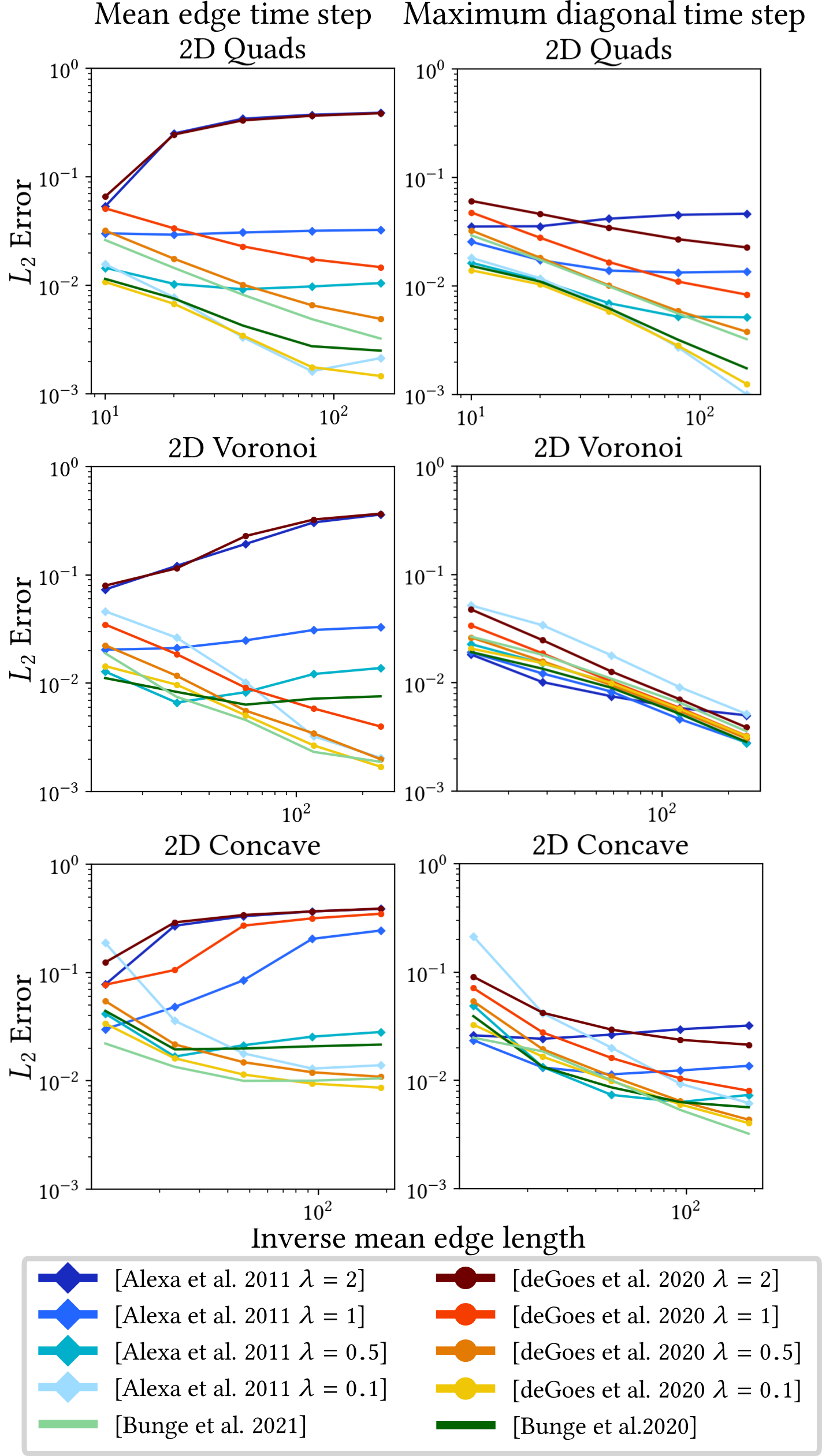
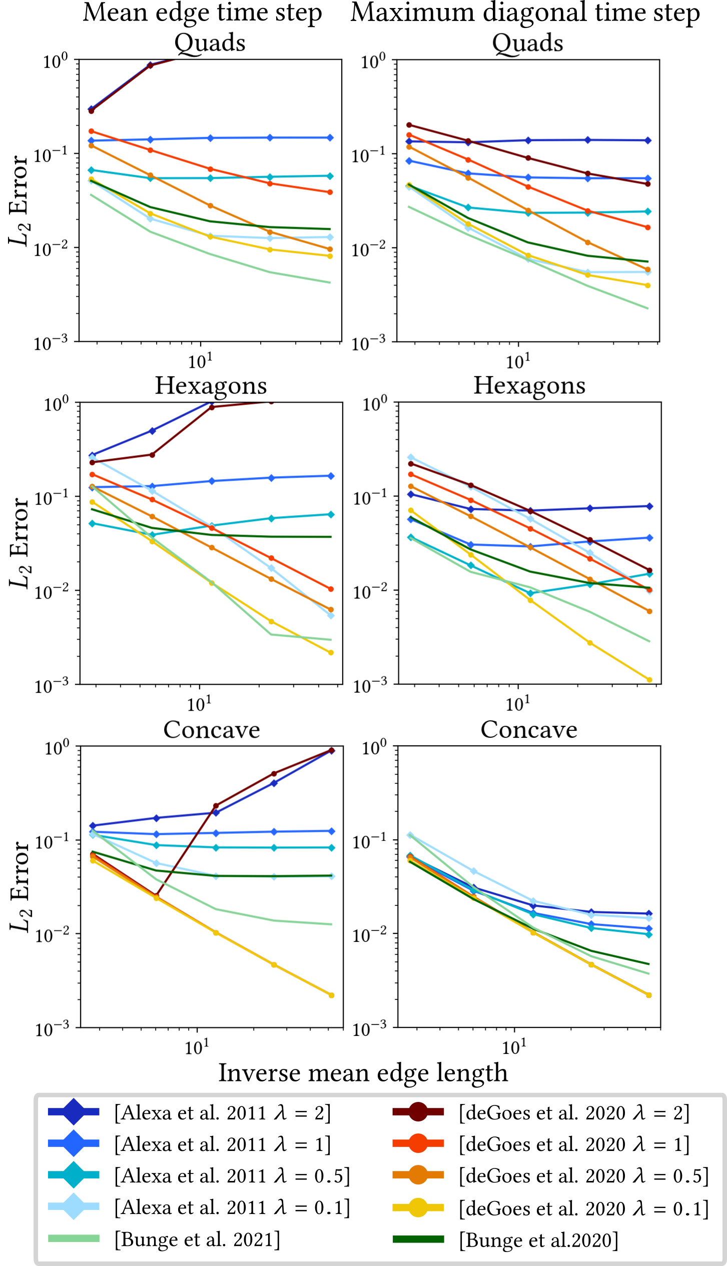
Timings and Sparsity
| Mesh | \(|\mathcal V|\) | [52] | [1] | [32] | [15] | [16] | ||||||||||
|---|---|---|---|---|---|---|---|---|---|---|---|---|---|---|---|---|
| build | nnz | solve | build | nnz | solve | build | nnz | solve | build | nnz | solve | build | nnz | solve | ||
| Quads 2D | 26k | 92s | 231k | 8ms | 44ms | 231k | 8ms | 47ms | 231k | 8ms | 10ms | 231k | 8ms | 43ms | 537k | 21ms |
| Voronoi 2D | 51k | 78s | 616k | 25ms | 94ms | 616k | 25ms | 76ms | 616k | 25ms | 29ms | 616k | 25ms | 224ms | 1723k | 74ms |
In this section, we compare different statistics involved in the solution process of a Poisson problem for 2D meshes. Table 1 lists the respective timings to construct the stiffness matrix (build), the number of its non-zero entries (nnz), and the time it takes to solve the system (solve) with Eigen’s SimplicialLLT solver [35]. The timings were measured on a standard workstation with a six-core Intel Xeon 3.6 GHz CPU. As discussed in the locality property section, all Laplacians, with the exception of the Diamond Laplacian, have the same sparsity pattern for their matrices, leading to roughly the same solving times. However, while the implementation of the respective methods has not been extensively optimized for efficiency, it is very apparent that the construction time of the harmonic shape functions by Martin et al. [52] exceeds the other operators by a tremendous amount. The time it takes to build the involved matrices makes the method not competitive, since its accuracy is on par with the linear virtual refinement method by Bunge et al. [15] and does not justify the large costs.
Mesh quality
An interesting sub-case of polygonal meshes are those with non-planar faces. They are in general more challenging than planar elements due to their twisted surfaces, but still occur frequently in computer graphics models. So far, we have only considered meshes with planar polygons in order to establish an intuition of the general effectiveness of each operator. However, in order to evaluate this more challenging setting of non-planar faces, we still have to retain a mesh with a known analytic solution to the given problem. We therefore added noise in tangential direction to the vertex positions of the previously mentioned hexagon spheres and projected them back onto the unit sphere. While this results in non-planar faces, note that the added noise also leads to less balanced hexagonal shapes. Equipped with these new test meshes, we repeat the spherical harmonics convergence test (see Figure 15). In general, each of the evaluated operators displays a higher error rate and slower convergence for the non-planar sphere, with the Laplacians presented by Bunge et al. [15, 16] being the least affected. In contrast to the planar case, choosing a lower hyperparameter \(\lambda\) for the operators of Alexa and Wardetzky [1] and de Goes et al. [32] leads to better results.
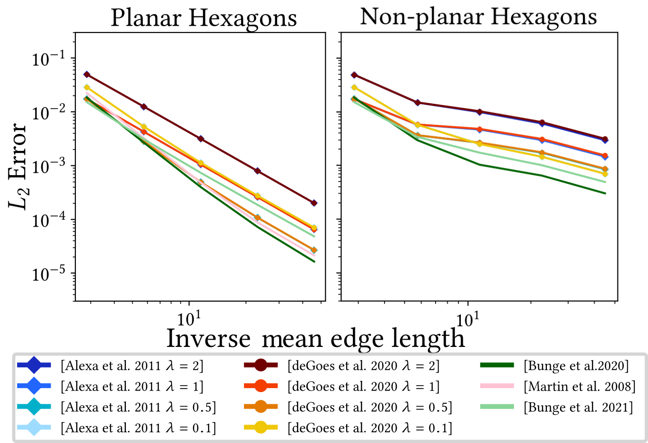
Similar tendencies can be observed if we add progressively stronger noise to the faces of a single mesh, as depicted in Figure 16. All operators display higher errors for increasingly twisted faces, but in this setting, choosing the same hyperparameter \(\lambda=0.5\) as in the planar case leads to the lowest rates for the works presented by Alexa and Wardetzky and de Goes et al. However, with increasing non-planarity the error converges to similar values as for \(\lambda=0.1\), which appears to be more stable. As in the other test, the operators presented by Bunge et al. lead to the lowest errors. The harmonic shape functions presented by Martin et al. [52] were not included in these evaluations, since their definition only holds for planar polygons.
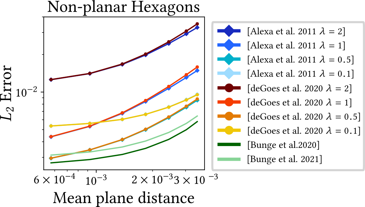
Another aspect in which the underlying tessellation may directly affect the quality of the operators is the shape of the faces itself. For example, Delaunay triangles lead to more favorable results and properties for the Laplacian than meshes consisting of less ideal triangulations [36]. A possible way to quantify the stability of the operator with respect to the given tessellation is to analyze its condition number \(\kappa\). It is defined as the ratio \[ \begin{equation} \label{eq:conditionNR} \kappa = \frac{\lambda_{max}}{\lambda_{min}} \end{equation} \] of the Laplacians largest and smallest non-zero eigenvalues \(\lambda_{max}\) and \(\lambda_{min}\). Note that the actual smallest eigenvalue would be zero, since the Laplacian has a one-dimensional kernel. The condition number gives us a notion about the numerical quality of the stiffness and mass matrices and the operators potential to quickly converge to the correct solution of a given problem [46]. We therefore evaluate the effect of decreasing polygon quality on the different Laplacians by incrementally collapsing a single edge of the previously considered quad plane, while measuring its effect on the respective condition numbers. The results can be seen in Figure 17.
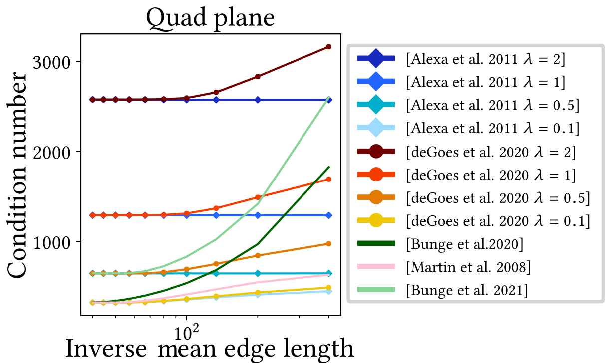
In general, all of the presented operators are not really affected by the first iterations of edge distortion. However, as the edge length approaches zero, the condition numbers of the Laplacians introduced by Bunge et al. [15, 16] begin to rise significantly due to the diminishing triangle quality of the virtual refinements. The numerical stability of the operators presented by Martin et al. [52] and de Goes et al. [32] also decreases, but with a lower magnitude. In contrast, the Laplacian presented by Alexa and Wardetzky [1] is not affected by the diminishing edge length and only slightly increases for the smallest hyperparameter \(\lambda=0.1\). However, both operators presented by Alexa and Wardetzky and de Goes et al. follow the pattern that a higher \(\lambda\) leads to generally larger condition numbers.
Summary and Recommendations
In light of the above, we want to summarize the presented results and give the reader a recommendation in which situation which operator should be used.
When only triangle meshes are concerned, the canonical choice is using the cotangent Laplacian. While most polygon Laplacians are identical to the cotangent Laplacian for triangle meshes, the direct implementation can be simpler and more performant. Furthermore, modifications, such as the intrinsic Delaunay triangulation [8], intrinsic mollification [65], or D-TFEM [73], can be added to significantly improve the robustness to (near-)degenerate geometry.
In the general polygon case, given their overall performance, the Laplacians presented by Alexa and Wardetzky and de Goes et al. lead to very favorable numerical results if the user is willing to adjust the stabilization parameter \(\lambda\). Furthermore, de Goes et al. provide a list of other operators that go hand in hand with the matrices introduced in this paper and lead to a larger variety of problems that can be handled with their method.
If the reader is looking for a method that leads to accurate results without any adjustments, the Diamond Laplacian would be their method of choice. However, given its denser matrix pattern, this approach leads to longer solving times.
If this is a problem, a computationally more efficient but slightly less accurate choice would be the operator presented by Bunge et al. [15]. Given that many applications already work with the cotangent Laplacian, it can be easily integrated since the only missing piece is the prolongation matrix. Furthermore, in the case of (near-)degenerate elements, it can be combined with modifications to the triangle Laplacian, such as intrinsic mollification [65] or D-TFEM [73].
The harmonic shape functions are not competitive in comparison to the other methods due to their costly construction process. However, they are able to reproduce P1 and Q1 elements on triangles and quads, are \(C^0\) continuous to P1/Q1 at the boundaries of polygons, and can therefore be seamlessly mixed with these standard elements.
Conclusion and Outlook
Throughout this tutorial, we attempted to give a comprehensive description of the recent advances achieved within the graphics community to construct robust discrete differential operators for any given manifold surface mesh. For triangle meshes, we observed that when computing the cotangent Laplacian, there is no clear winner when robust implementation is concerned. Both extrinsic and intrinsic formulations have individual strengths on different types of triangles, whereas purely trigonometric approaches generally perform poorly in comparison. Regardless, clamping of negative weights should be avoided, while ignoring (close-to-)zero-area triangles is often beneficial. Furthermore, using non-standard methods like mollification [65], intrinsic Delaunay triangulation [8] (in combination with mollification), or D-TFEM [73] can dramatically reduce errors and, in most cases, provide a solvable system across a wide range of meshes.
In the second part of the tutorial, we examined the numerical schemes used for the respective polygon Laplacians, providing context for the individual discretization strategies and motivating the problems involved in their generalization process. Furthermore, we analyzed the properties of the presented Laplacians and investigated similarities and parallels between the different methods. Additionally, we introduced a variety of discrete gradient and divergence operators and explained the relationship to their associated Laplacian. Finally, we provide a list of quantitative comparisons between the presented operators that highlight their individual strengths and weaknesses while simultaneously addressing recurring debates within the original papers.
Overall, we hope this tutorial encourages the use of more challenging triangle meshes and general tessellations within the graphics community, given that the necessary tools for many applications are already available. Furthermore, besides the Laplacian, gradient, and divergence, there exist a variety of other discrete differential operators that could be useful to the graphics community, as touched upon by de Goes et al. [32] and Lipnikov et al. [49] in their survey on the MFD method.
Acknowledgements
We are grateful to Marc Alexa and Philipp Herholz for their help and support during the whole project. Thank you to Olga Sorkine-Hornung and Misha Kazhdan for all the valuable discussions about polygon shape functions and their properties. Finally, we are grateful to Fernando de Goes and Max Wardetzky for providing feedback on the implementation of the respective Laplacians. This research has been supported by the Federal Ministry of Education and Research of Germany and the state of North Rhine-Westphalia as part of the Lamarr Institute for Machine Learning and Artificial Intelligence.