A Hands-On Introduction to Discrete Differential Operators on Polygon Meshes
Other Laplacians on Polygon Meshes

Sven D. Wagner
TU Dortmund

Astrid Bunge
AutoForm Engineering

Mario Botsch
TU Dortmund

Generalized Barycentric Coordinates
- Wachspress Coordinates
- Wachspress, Warren
- Mean Value Coordinates
- Floater, Hormann, Ju, Wicke
- Maximum Entropy Coordinates
- Sukumar, Hormann
- Harmonic Coordinates
- Joshi, Martin
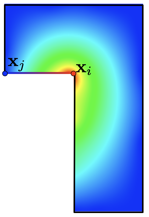
Poisson System on 2D Voronoi Meshes
13.5053,	28.5194,	58.8386,	119.78,	241.153
Standard LVR, 0.00768401,0.00193955,0.00057802,0.000152567,3.41754E-05
Harmonic,	0.00951959,	0.00236579,	0.000699382,	0.000188646,	5.46139E-05
Robust LVR ,	0.00795767, 0.00198379 , 0.000572063, 0.000147802,3.33787E-05


<!--
{
  "options": {
    "scales": {
      "x": {
        "title": {
          "text": "inverse mean edge length",
          "display": true
        },
        "type": "logarithmic"
      },
      "y": {
        "title": {
          "text": "L2 error",
          "display": true
        },
        "type": "logarithmic"
      }
    }
  }
}
-->
Expected convergence rate 😄 Expensive to compute, evaluate, and integrate 😢

DEC Polygon Laplacians
- Generalize DEC to non-planar polygons
- Discretization of \(\laplace f = \delta d f\) (Laplace-de Rham)
- The exterior derivative \(d\) becomes the difference operator \(\mat{d}\)
- The co-differential \(\delta\) can be discretized as \(\mat{M}_0^{-1} \mat{d}\T \mat{M}_1\)
- Putting it together: \(\laplace \vec{u} \;\approx\; -\mat{M}_0^{-1} \mat{d}\T \mat{M}_1 \mat{d}\, \vec{u}\)
Difference operator
- The difference operator maps
- From values on vertices (0-forms)

Difference operator
- The difference operator maps
- From values on vertices (0-forms)
- To differece values on (half-)edges (1-forms)

Poisson System on 2D Voronoi Meshes
13.5053,	28.5194,	58.8386,	119.78,	241.153
Alexa11; λ=2,	0.00838748,	0.00209687,	0.000476346,	0.000127937,	3.30444E-05
Alexa11; λ=1,	0.00456036,	0.0010483,	0.000382806,	8.53325E-05,	1.84683E-05
Alexa11; λ=0.5,	0.00800984,	0.00193734,	0.000621653,	0.000143936,	3.19937E-05
Alexa11; λ=0.1,	0.0144414,	0.00337097,	0.000947331,	0.000221091,	5.14271E-05
deGoes20; λ=2,	  0.00965471,	0.00245388,	  0.000542276,	0.000145297,	3.74297E-05
deGoes20; λ=1,	  0.00435302,	0.000996788,	0.000354402,	7.95537E-05,	1.73643E-05
deGoes20; λ=0.5,	0.00747841,	0.00182759,	  0.00059557,	  0.000138136,	3.05869E-05
deGoes20; λ=0.1,	0.0139834,	0.00327528,	  0.00092799,	  0.000217473,	5.03785E-05
<!--
{
  "options": {
    "scales": {
      "x": {
        "title": {
          "text": "inverse mean edge length",
          "display": true
        },
        "type": "logarithmic"
      },
      "y": {
        "title": {
          "text": "L2 error",
          "display": true
        },
        "type": "logarithmic"
      }
    }
  }
}
-->
Poisson System on 2D Voronoi Meshes
13.5053,	28.5194,	58.8386,	119.78,	241.153
Standard LVR, 0.00768401,0.00193955,0.00057802,0.000152567,3.41754E-05
Harmonic,	0.00951959,	0.00236579,	0.000699382,	0.000188646,	5.46139E-05
Alexa11; λ=1,	0.00456036,	0.0010483,	0.000382806,	8.53325E-05,	1.84683E-05,
Alexa11; λ=0.1,	0.0144414,	0.00337097,	0.000947331,	0.000221091,	5.14271E-05
deGoes20; λ=1,	  0.00435302,	0.000996788,	0.000354402,	7.95537E-05,	1.73643E-05
deGoes20; λ=0.1,	0.0139834,	0.00327528,	  0.00092799,	  0.000217473,	5.03785E-05

<!--
{
  "options": {
    "scales": {
      "x": {
        "title": {
          "text": "inverse mean edge length",
          "display": true
        },
        "type": "logarithmic"
      },
      "y": {
        "title": {
          "text": "L2 error",
          "display": true
        },
        "type": "logarithmic"
      }
    }
  }
}
-->
Discrete Duality Finite Volumes (DDFV)


Quiz
How do we get diamond cells on an arbitrary polygon mesh?


2D DDFV
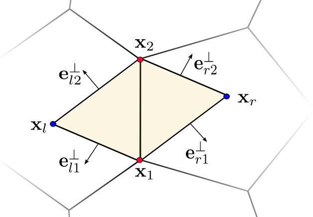
\[ \grad u|_D \;=\; \frac{1}{2 \abs{D}} \sum_{(i,j) \in \partial D} \vec{e}_{ij}^\perp \frac{u_i+u_j}{2} \]
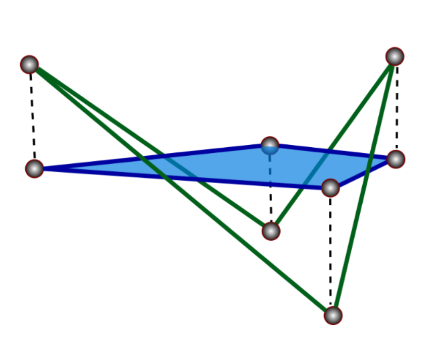
Virtual Dual Vertices
 \[\downarrow\]
  \[\downarrow\]
- Combine ideas from DDFV and virtual refinement
- Use virtual vertices as dual mesh
- Compute DDFV operator on the “virtual diamonds”
- Express diamond in an intrinsic 2D coordinate system
- Restrict values back to the original mesh
Poisson System on 2D Voronoi Meshes
13.5053,	28.5194,	58.8386,	119.78,	241.153
Standard LVR, 0.00768401,0.00193955,0.00057802,0.000152567,3.41754E-05
Harmonic,	0.00951959,	0.00236579,	0.000699382,	0.000188646,	5.46139E-05
Alexa11; λ=1,	0.00456036,	0.0010483,	0.000382806,	8.53325E-05,	1.84683E-05
deGoes20; λ=1,	  0.00435302,	0.000996788,	0.000354402,	7.95537E-05,	1.73643E-05
Diamond, 0.00610683,0.00155889,0.000413685,0.000105977,2.46064E-05
<!--
{
  "options": {
    "scales": {
      "x": {
        "title": {
          "text": "inverse mean edge length",
          "display": true
        },
        "type": "logarithmic"
      },
      "y": {
        "title": {
          "text": "L2 error",
          "display": true
        },
        "type": "logarithmic"
      }
    }
  }
}
-->
Poisson System on 2D Meshes
13.5053,	18.8048, 24.0398 , 37.072 ,50.2679
Robust LVR ,	0.00745003, 0.0036901, 0.00222217 , 0.000924393 , 0.000501055
Standard LVR,	0.0385146, 0.0226358, 0.0147572, 0.00647153, 0.00376134
Alexa11; λ=2, 0.0611674, 0.041198, 0.0291081, 0.0144778, 0.00876606
Alexa11; λ=0.5, 0.01545 , 0.00859024 , 0.00546532 , 0.0023337,0.00132841
deGoes20; λ=1, 0.0363144 , 0.0221452, 0.0148121, 0.00684791, 0.00400674
deGoes20; λ=0.1, 0.0252731, 0.0122202, 0.00700861, 0.00268186, 0.00139388
Diamond, 0.0131201, 0.00576263 , 0.0029424, 0.00113579 , 0.00071783
<!--
{
  "options": {
    "scales": {
      "x": {
        "title": {
          "text": "inverse mean edge length",
          "display": true
        },
        "type": "logarithmic"
      },
      "y": {
        "title": {
          "text": "L2 error",
          "display": true
        },
        "type": "logarithmic"
      }
    }
  }
}
-->

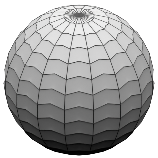
Poisson System on Sphere Meshes
2.76125, 6.02378, 12.5599, 25.6378, 51.7971
Robust LVR , 0.0195403, 0.00757413, 0.00353687, 0.00173384, 0.000859737
Standard LVR,	 0.0292485, 0.0119197, 0.00558098, 0.00270908, 0.00133463
Alexa11; λ=2, 0.0893085, 0.0490686, 0.0258716, 0.0131541, 0.00660642
Alexa11; λ=0.5, 0.0138582, 0.00877119, 0.00489306, 0.00251059, 0.00126177
deGoes20; λ=1, 0.0500151, 0.0278916, 0.0147208, 0.00751131, 0.00378149
deGoes20; λ=0.1, 0.0267659, 0.0115076 , 0.00583512 , 0.00289191, 0.00143387
Diamond, 0.024761, 0.00765354, 0.00354862, 0.0017351, 0.000857455
<!--
{
  "options": {
    "scales": {
      "x": {
        "title": {
          "text": "inverse mean edge length",
          "display": true
        },
        "type": "logarithmic"
      },
      "y": {
        "title": {
          "text": "L2 error",
          "display": true
        },
        "type": "logarithmic"
      }
    }
  }
}
-->
Computational Performance

Conclusion
- Gave a hands on introduction to Cotan Laplacian
- Discussed its derivation and several applications
- Showed methods to avoid numerical pitfalls on bad triangles
- Presented recent progress for Polygon Laplacians
- Discuss individual discretization strategies
- Analyze strength and weaknesses

- Acknowledgments
- Collaborators: Marc Alexa, Philipp Herholz, Misha Kazhdan, Olga Sorkine-Hornung
- Code-Checkers: Fernando de Goes, Max Wardetzky