A Hands-On Introduction to Discrete Differential Operators on Polygon Meshes

Applications II: Geodesics in Heat

Sven D. Wagner

TU Dortmund

Astrid Bunge

AutoForm Engineering

Mario Botsch

TU Dortmund

🚀 by Decker

Gradient and Divergence

\[\laplace f = \div(\nabla f) \Leftrightarrow \mat L = \mat D \cdot \mat G\]

Gradient and divergence are also important in geometry processing
- Many different applications need them

Gradient-based deformation

images/wildDDG/deformed_cylinder_tfem.png

Gradient-based deformation
Geodesic Distances

Gradient and Divergence on Triangle Meshes

\(f(\mathbf x) = \sum_{i\in\mathcal V} f_i \varphi_i(\vec x)\) \(\quad\Leftrightarrow\quad\nabla f(\mathbf x) = \sum_{i\in\mathcal V} f_i \nabla \varphi_i(\mathbf x)\)

\(\nabla \varphi_i(\mathbf x)\) is piece-wise constant (i.e., constant per triangle)

Gradient Operator \(\mathbf G \in \R^{3|\mathcal T| \times |\mathcal V|}\)

Mapping from vertex-based scalar field to triangle-based gradient field
- Built from local per-triangle matrices \(\mat G_i \in \R^{3\times 3}\) with

\[\mat G_i(:,1) = \nabla \varphi_j(\vec x)\Big\vert_{t_{jkl}} = \frac{(\mathbf x_l - \mathbf x_k)^\bot}{2|t_{jkl}|}\]

Divergence Operator \(\mathbf D = \mat G^\top \hat{\mat M} \in \R^{|\mathcal V| \times 3|\mathcal T|}\)

Gradient and Divergence on Polygon Meshes

\[\begin{align*} \mat L &= \mat P^\top \mat L^{\mathrm{tri}} \mat P\\ &= \mat P^\top \mat D^{\mathrm{tri}} \mat G^{\mathrm{tri}} \mat P \end{align*}\]

Gradient and divergence are based on virtual triangles:

\[\begin{align*} \mat G &= \mat G^{\mathrm{tri}} \mat P\\ \mat D &= \mat P^\top \mat D^{\mathrm{tri}} \end{align*}\]

Can also be made robust using D-TFEM 👍

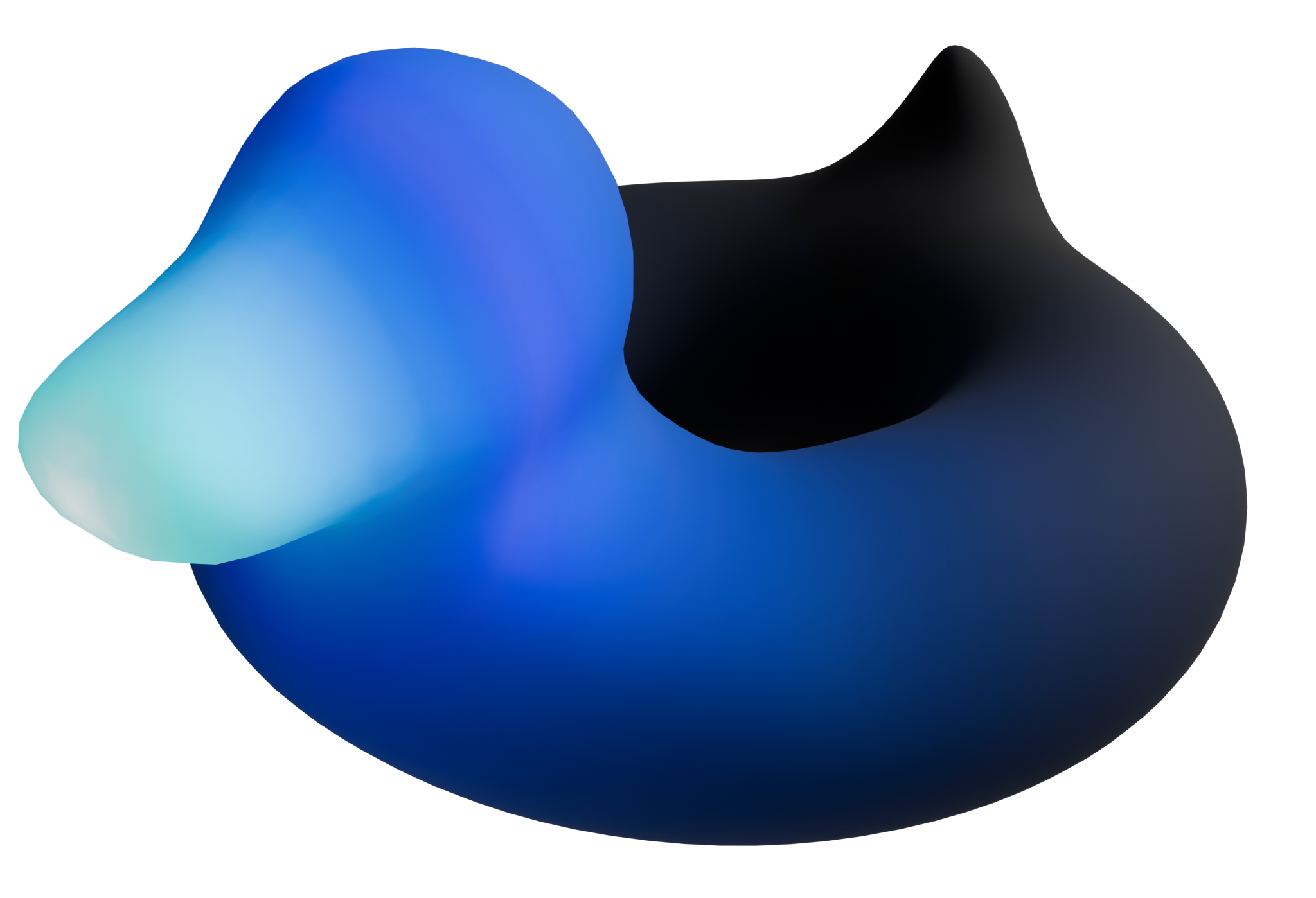
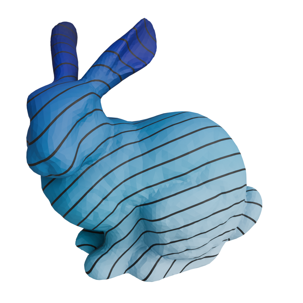
Geodesics in Heat

We want to know the distance from a given vertex \(v_i\) to all other vertices

Approximate geodesic distances using heat diffusion
- Idea: Both have similar normalized gradient fields

Calculate heat flow for given time step \(t\)
- Solve implicit time integration problem \((\mat M - t \mat L) \vec u = \delta_i\)

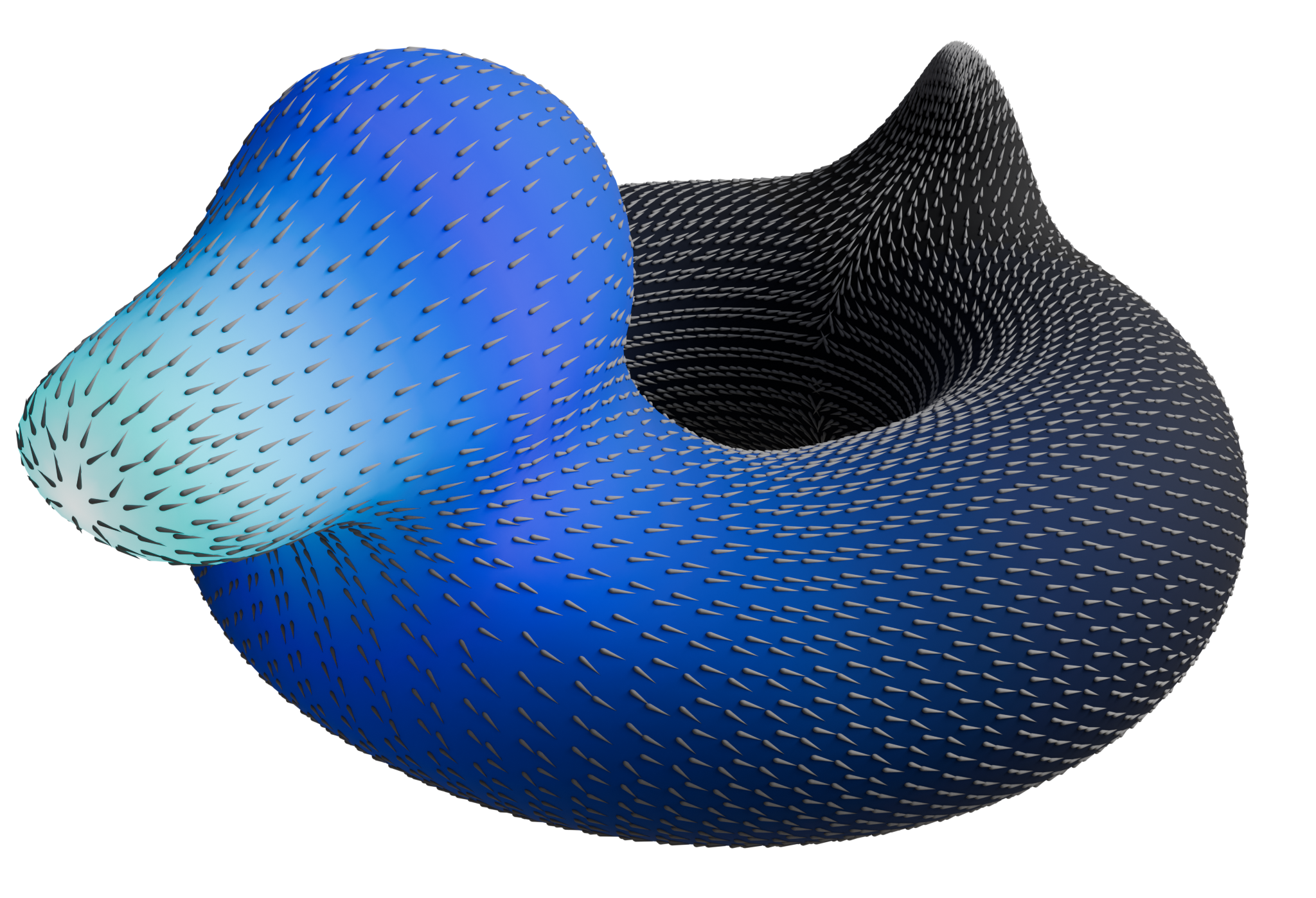
Evaluate normalized gradient field
- Compute vector field \(\vec g_j = -(\mat G \vec u)_j / ||(\mat G \vec u)_j||\)

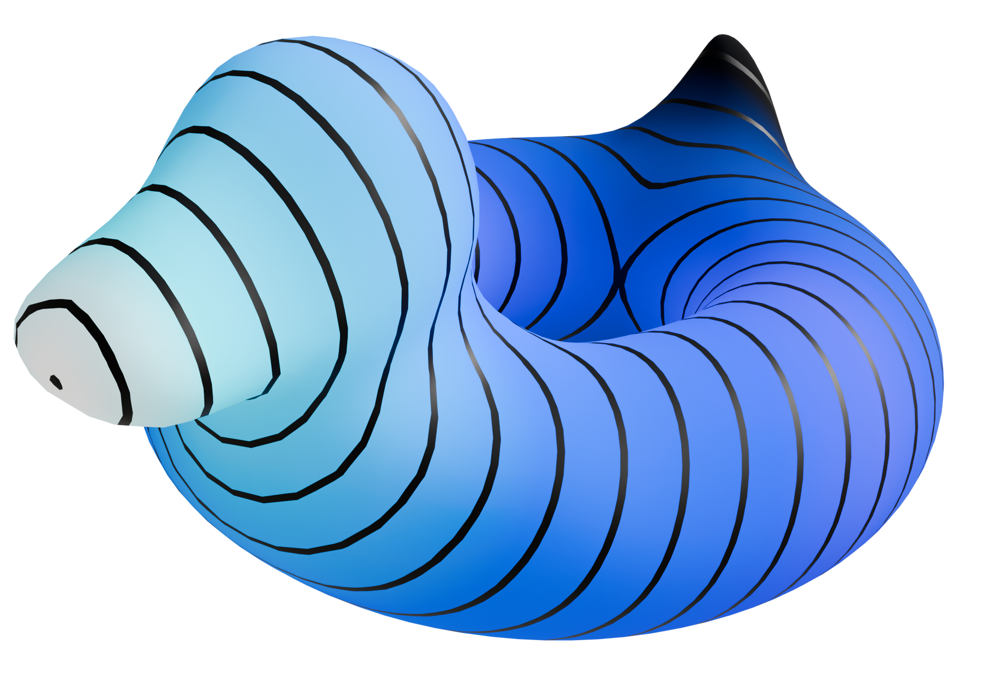
Solve for scalar potential with closest gradient field
- Solve Poisson equation \(\mat L \, \vec d = \mat D \, \vec g\)

\(\vec d\) contains geodesic distances from \(v_i\) 👍

Let’s Get to Coding 💻

References

Bunge, Astrid, Philipp Herholz, Misha Kazhdan, and Mario Botsch. 2020. “Polygon Laplacian Made Simple.” Computer Graphics Forum 39 (2).

Crane, Keenan, Clarisse Weischedel, and Max Wardetzky. 2013. “Geodesics in Heat: A New Approach to Computing Distance Based on Heat Flow.” ACM Transactions on Graphics 32 (5): 152:1–11.

Wagner, Sven Dominik, and Mario Botsch. 2025. “Robust Discrete Differential Operators for Wild Geometry.” In Vision, Modeling, Visualization.